5. Amortization: Amortized Analysis

What this lecture covers

The lecture answers how to bound the total running time of a sequence of data structure operations when individual operations can occasionally be expensive. Rather than proving a worst-case bound per operation, amortized analysis proves a bound on the average cost over a whole sequence, which is what actually matters in algorithms like Dijkstra's that only care about total running time.

This is the fifth lecture in MIT's Design and Analysis of Algorithms course. Professor Demaine presents four methods for amortized analysis — aggregate, accounting, charging and potential — and applies them to table doubling, binary counters, 2-3 trees and 2-5 trees. After watching, you should be able to choose an appropriate method for a given problem and construct a potential function or charging scheme to prove a constant or logarithmic amortized bound.

Key ideas

• Amortized cost: an assignment of cost to each operation in a sequence such that the sum of amortized costs is always at least the sum of actual costs, so bounding amortized cost bounds total cost even though individual operations can still be expensive.
• Aggregate method: sum the actual costs of a sequence of operations and divide by the number of operations; simple but only works cleanly when the sequence of operation types is fixed or easy to bound, as in table doubling with insertions only.
• Accounting method: maintain a non-negative bank balance where cheap operations deposit credit and expensive operations withdraw it; for example, in a 2-3 tree, each insertion deposits O(log n) credit so later deletions can be charged for free.
• Charging method: let an expensive operation retroactively charge part of its cost to earlier operations since the last similarly expensive operation, as long as no earlier operation is ever charged twice; used to show table doubling and halving cost constant amortized time per insert or delete.
• Potential method: define a potential function of the current data structure state (always non-negative, typically zero for the empty structure) so that amortized cost equals actual cost plus the change in potential; the sum telescopes, so bounding each operation's amortized cost bounds the total.
• Binary counter increments: using the number of 1-bits as the potential function shows that incrementing a binary counter costs O(1) amortized time, even though a single increment can flip many bits.
• 2-3 tree splits: counting the number of 3-nodes as potential shows that insertion-only 2-3 trees do O(1) amortized splits per insertion, even though a single insertion can cascade splits up to O(log n) levels.
• 2-5 trees for insert and delete: ordinary 2-3 trees do not give constant amortized cost once deletions are mixed in; using nodes with 2 to 5 children and counting nodes with 2 or 5 children as potential gives O(1) amortized cost for both insert and delete.

Walkthrough

Motivation and the aggregate method (0:00)

The lecture opens by connecting amortization to algorithms like Dijkstra's, where only the total running time of the data structure operations matters, not each individual cost. The table-doubling example from hash tables is revisited: doubling a table costs O(size), but it only happens O(log n) times over n insertions, and summing the geometric series shows the total cost for n insertions is O(n), giving O(1) amortized cost per insertion. This is the aggregate method — sum total costs and divide by the number of operations.

The general definition and 2-3 tree example (7:08)

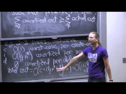
The lecture generalizes to a formal definition: amortized costs are valid whenever their sum is at least the sum of actual costs. Using a 2-3 tree with O(1) creation, O(log n) insertion and free deletion as an example, it shows that since the number of deletions can never exceed the number of insertions, charging zero to deletions and 2 log n to insertions still bounds the total actual cost.

Accounting method: bank balances and coins (13:11)

The accounting method treats each operation as able to deposit or withdraw credit from a bank balance that must stay non-negative. Applied to 2-3 trees, each insertion deposits a coin of value log i (where i is the item's insertion rank), and deletions withdraw the corresponding coin. Applied to table doubling, the lecture places a physical coin on each inserted item and shows that by the time the table is full, the most recently inserted half of the items hold enough coins to pay for the next doubling.

Charging method: billing the past (27:54)

The charging method lets an expensive operation retroactively bill part of its cost to earlier, related operations, as long as no operation is charged more than once. For table doubling and halving together (doubling at 100% full, halving at 25% full, so the table is always 50% full right after a resize), each doubling is charged to the Θ(size) insertions since the last resize, and each halving to the Θ(size) deletions since the last resize, giving O(1) amortized cost per insert or delete.

Potential method and binary counters (41:21)

The potential method defines a non-negative function of the data structure's state; amortized cost is actual cost plus the change in potential, and the sum telescopes over a sequence of operations. Applied to incrementing a binary counter, using the number of trailing ones as potential fails, but using the total number of 1-bits works: an increment destroys some number of 1-bits and creates at most one, so the amortized cost of an increment is O(1).

2-3 tree splits with the potential method (55:54)

Reanalyzing insertion-only 2-3 trees with the potential method, the number of 3-nodes serves as the potential function. Each split converts a 3-node into two 2-nodes, decreasing potential by one, while at most one new 3-node is created when splitting stops, so K splits during an insertion have amortized cost K - K + 1 = 1.

2-5 trees for insert and delete (1:04:20)

Because inserting and deleting from an ordinary 2-3 tree can force Θ(log n) cascading splits or merges per operation, the lecture introduces 2-5 trees, where nodes have between 2 and 5 children. Using the number of nodes with exactly 2 or exactly 5 children as the potential function, splits (from overfull 5-nodes) and merges (from underfull 2-nodes) each reduce potential enough to give O(1) amortized cost per insert or delete. The lecture notes this generalizes to any AB-tree where a is strictly less than b/2.

Before you watch

• Review hash table doubling and 2-3 trees, which recur throughout the lecture as running examples.
• Basic familiarity with geometric series is useful for following the aggregate method's proof that table doubling costs O(n) total.

Check your understanding

1. Why does the aggregate method work cleanly for insertion-only table doubling but require more care once deletions are mixed in?
2. In the accounting method's coin-based analysis of table doubling, why must at least half the items hold unused coins by the time the table is full?
3. Why does counting the total number of 1-bits (rather than trailing ones) give a working potential function for binary counter increments?
4. Why do 2-3 trees fail to give constant amortized cost once both insertions and deletions occur, and how do 2-5 trees fix this?