Lecture 4: Perceptron, GLMs, and Softmax Regression

What this lecture covers

Taught by head TA Anand Avati, this lecture briefly introduces the perceptron algorithm, then spends most of its time building generalized linear models (GLMs) from exponential family distributions, showing that linear regression and logistic regression are both special cases. It closes with softmax regression for multi-class classification, derived through cross-entropy minimization rather than the GLM framework.

This follows directly from the previous lecture's logistic regression and sets up why the update rules for linear and logistic regression look so similar. After watching, you should be able to write the exponential family form of a distribution, explain the three GLM design assumptions, and describe how softmax regression generalizes logistic regression to multiple classes.

Key ideas

• Perceptron algorithm: uses a hard threshold, g(z) = 1 if z >= 0 else 0, instead of the sigmoid; its update rule has the same form as logistic regression's but is not derived from a probabilistic model, and is taught mainly for historical interest.
• Exponential family: a class of probability distributions whose density can be written as b(y) * exp(eta*T(y) - a(eta)), where eta is the natural parameter, T(y) the sufficient statistic (often just y), b(y) the base measure, and a(eta) the log-partition function.
• Bernoulli and Gaussian as exponential family members: algebraic rearrangement shows the Bernoulli's natural parameter is log(phi/(1-phi)) and a fixed-variance Gaussian's natural parameter is its mean mu.
• Generalized linear model (GLM) assumptions: y given x follows an exponential family distribution, the natural parameter eta = theta^T*x, and the prediction at test time is the distribution's mean.
• Three parameterizations: model parameters (theta, learned by gradient ascent), the natural parameter (eta, linked to theta by eta = theta^T*x), and canonical parameters (like phi, mu, or lambda, linked to eta by the canonical response function).
• Universal GLM update rule: regardless of which exponential family distribution is chosen, the gradient ascent update is theta_j := theta_j + alpha*(y_i - h_theta(x_i))*x_ij, with only h_theta(x) changing.
• Softmax regression: a multi-class generalization of logistic regression with one parameter vector per class, converting per-class linear scores into a probability distribution via exponentiation and normalization, trained by minimizing cross-entropy between the predicted and true (one-hot) label distributions.

Walkthrough

The perceptron algorithm (3:22)

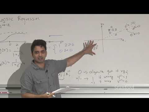
Avati contrasts the perceptron with logistic regression: instead of the sigmoid, it uses a hard step function that outputs exactly 0 or 1. Both share the same-looking update rule, theta_j := theta_j + alpha*(y_i - h_theta(x_i))*x_ij, though h_theta(x) means something different in each. Geometrically, when the perceptron misclassifies an example, it nudges the decision boundary's normal vector theta toward (or away from) that example's feature vector, using the intuition that similar vectors have positive dot products. The perceptron is taught mainly for historical reasons: it lacks a probabilistic interpretation and, as Marvin Minsky showed, cannot separate certain simple datasets.

Exponential family distributions (12:27)

Avati defines the exponential family form p(y; eta) = b(y) * exp(eta*T(y) - a(eta)), where y is the data, eta the natural parameter, T(y) the sufficient statistic (equal to y in the distributions covered), b(y) the base measure, and a(eta) the log-partition function (the log of the normalizing constant). He shows, through algebraic rearrangement, that the Bernoulli distribution fits this form with eta = log(phi/(1-phi)), which inverts to the sigmoid function, and that a fixed-variance Gaussian fits it with eta = mu. Useful properties follow from this form: under the natural parameterization, maximum likelihood estimation is concave (so negative log-likelihood is convex), and the mean and variance of the distribution can be obtained by differentiating a(eta) once and twice, rather than integrating.

Generalized linear models: three parameterizations (35:47)

A GLM extends the exponential family to include input features through three design choices: y given x (parameterized by theta) is a member of an exponential family; the natural parameter is set to eta = theta^T*x; and the model's prediction is the mean of that distribution. Avati distinguishes three parameter spaces: the model parameters theta that are actually learned by gradient ascent, the natural parameter eta linked to theta linearly, and the canonical parameters of the chosen distribution (phi for Bernoulli, mu and sigma^2 for Gaussian, lambda for Poisson), linked to eta through the canonical response function g (the derivative of the log-partition function) and its inverse, the canonical link function. Regardless of which exponential family distribution is chosen, the gradient ascent update rule for theta takes the same form, differing only in the definition of h_theta(x), which is why linear and logistic regression share an update rule.

Recovering linear and logistic regression from GLMs (1:01:53)

Avati works through the data-generating story behind each choice of distribution. For regression, assuming y given x is Gaussian with mean theta^T*x and fixed variance means each training point is imagined as sampled from a Gaussian centered on a line, and fitting theta amounts to finding the line the data was most likely sampled from, exactly linear regression. For classification, assuming a Bernoulli distribution whose parameter phi is obtained by passing eta = theta^T*x through the sigmoid recovers logistic regression, showing that the sigmoid isn't an arbitrary choice but falls out naturally from choosing a Bernoulli output distribution within the GLM framework.

Softmax regression for multi-class classification (1:08:30)

For classification into more than two classes, Avati introduces softmax regression with one parameter vector theta_class per class (k classes total), where labels are one-hot vectors. For a given input x, each class's linear score theta_class^T*x (called a "logit") is exponentiated to make it positive, then normalized by the sum across all classes, producing a probability distribution over classes. Geometrically, each class's boundary is a hyperplane, and softmax converts the resulting real-valued scores into class probabilities.

Cross-entropy loss (1:19:55)

Training minimizes the cross-entropy between the predicted probability distribution and the true one-hot label distribution, sum(p(y) * log(p_hat(y))) over classes, which simplifies to the negative log-probability the model assigns to the correct class. Avati writes out this loss for softmax regression explicitly and notes it is minimized with gradient descent with respect to the per-class parameters, arriving at the same style of optimization used throughout the lecture.

Before you watch

• Watch Lecture 3 first for logistic regression and maximum likelihood estimation, both assumed here.
• Comfort with partial derivatives and basic probability (density functions, expectation) makes the exponential family derivations much easier to follow.

Check your understanding

1. Why does the lecture say the perceptron's update rule looks like logistic regression's but lacks a probabilistic interpretation?
2. What are the three design assumptions that turn an exponential family distribution into a generalized linear model?
3. Why does the same gradient ascent update rule work for both linear regression and logistic regression under the GLM framework?
4. How does softmax regression convert a set of per-class linear scores into a valid probability distribution over classes?