Lecture 3: Locally Weighted and Logistic Regression

What this lecture covers

This lecture extends last time's linear regression into three directions. First, locally weighted regression, a non-parametric method that fits curved data without hand-picking polynomial features. Second, a probabilistic justification for why linear regression minimizes squared error. Third, the course's first classification algorithm, logistic regression, along with Newton's method as a faster alternative to gradient ascent for finding its parameters.

This sits right after linear regression and gradient descent in the course, and its probabilistic framing sets up generalized linear models, covered next. After watching, you should be able to explain why locally weighted regression is non-parametric, derive the least-squares cost function from a Gaussian noise assumption, write the logistic regression hypothesis and its update rule, and describe how Newton's method differs from gradient ascent.

Key ideas

• Locally weighted regression: fits a separate local line for each prediction point, weighting nearby training examples heavily and distant ones near zero, so it can trace curved data without you choosing polynomial features.
• Parametric vs. non-parametric algorithms: a parametric algorithm (like ordinary linear regression) fits a fixed-size set of parameters and can then discard the data; a non-parametric algorithm (like locally weighted regression) needs to keep data around, and the amount of storage grows with the training set.
• Bandwidth parameter tau: controls how wide the weighting function is in locally weighted regression, trading off overfitting a jagged fit against oversmoothing the data.
• Probabilistic justification of least squares: assuming prediction errors are independently and identically distributed (IID) Gaussian noise, maximizing the likelihood of the data is mathematically the same as minimizing the squared-error cost function.
• Logistic regression: a classification algorithm that passes theta^T * x through the sigmoid function g(z) = 1/(1+e^-z) so the hypothesis output lies between 0 and 1, interpreted as P(y=1|x).
• Maximum likelihood estimation (MLE): choosing parameters theta that maximize the probability of the observed data; used to derive the update rules for both linear and logistic regression.
• Newton's method: an iterative root-finding method that uses the tangent line at the current point to jump to the next estimate, converging in far fewer iterations than gradient ascent but with a more expensive step (it requires inverting a Hessian matrix).

Walkthrough

Locally weighted regression (5:07)

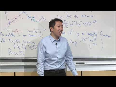
After recapping last lecture's notation, Ng poses the problem of fitting curved data. Rather than manually choosing polynomial features like x^2 or sqrt(x), locally weighted regression fits a fresh straight-line regression for each point where you want a prediction, focusing on training examples close to that point. The cost function is modified with a weight w^(i) for each example, commonly a bell-shaped (though not Gaussian) function of the distance between that example's input and the query point: weight near 1 for close examples, near 0 for distant ones.

Non-parametric learning and the bandwidth parameter (5:53)

Ng contrasts parametric algorithms, which fit a fixed set of parameters and can then discard the training data, with non-parametric algorithms like locally weighted regression, where the amount of data you must keep grows with the training set size. He introduces the bandwidth parameter tau, which controls how wide the local weighting window is: too wide oversmooths the data, too narrow produces a jagged, overfit curve. He notes that locally weighted regression works well when the number of features is small but you have plenty of data, and that it becomes computationally expensive at very large scale, where methods like KD-trees help.

Probabilistic interpretation of linear regression (21:32)

To justify the earlier choice of squared error, Ng assumes each house's true price is theta^T * x plus an error term that is IID Gaussian with mean 0 and variance sigma^2. This implies y given x and theta is Gaussian with mean theta^T * x. Writing out the likelihood of the parameters as the product of these Gaussian densities over all training examples (using the IID assumption), and taking the log-likelihood, he shows that maximizing this log-likelihood is equivalent to minimizing the same squared-error cost function J(theta) from the previous lecture. In other words, least squares falls out naturally from assuming Gaussian, independent errors, which by the central limit theorem is a reasonable default when errors are the sum of many small, uncorrelated effects.

Logistic regression (46:18)

Ng first shows why applying linear regression directly to a 0/1 classification problem is a bad idea: a single added training example far from the rest can shift the fitted line enough to flip the decision threshold at 0.5, and the output isn't naturally bounded to [0, 1]. Logistic regression instead passes theta^T * x through the sigmoid (logistic) function, g(z) = 1/(1+e^-z), so h(x) always lies between 0 and 1 and is interpreted as P(y=1|x; theta), with P(y=0|x; theta) = 1 - h(x). Both cases combine into a single expression, P(y|x; theta) = h(x)^y * (1-h(x))^(1-y), which makes it possible to write the likelihood of the parameters as a product over training examples and derive its log-likelihood. Maximizing this log-likelihood with batch gradient ascent produces an update rule for theta that looks algebraically identical in form to linear regression's gradient descent rule, differing only in the definition of h(x) and the sign (ascent versus descent). Ng notes the log-likelihood surface for logistic regression is concave, so gradient ascent always converges to a global maximum, and that, unlike linear regression, logistic regression has no closed-form normal equation.

Newton's method (1:05:57)

As a faster alternative to gradient ascent, Ng introduces Newton's method for finding a value of theta where a function f(theta) equals zero, which can be applied to logistic regression by setting f to the derivative of the log-likelihood. Each iteration draws the tangent line to f at the current point and jumps to where that line crosses zero, giving the update theta := theta - f(theta)/f'(theta). For a vector-valued theta, this generalizes to theta := theta - H^-1 * gradient, where H is the Hessian matrix of second derivatives. Newton's method exhibits quadratic convergence, roughly doubling the number of correct digits each iteration, so it typically needs far fewer iterations than gradient ascent. Its downside is that each step requires inverting a matrix the size of the parameter vector, which becomes expensive when there are many parameters; Ng's rule of thumb is to prefer Newton's method for tens or low hundreds of parameters and gradient descent for tens of thousands or more.

Before you watch

• Watch Lecture 2 first for the linear regression hypothesis, cost function, and gradient descent notation this lecture builds on directly.
• A working knowledge of probability density functions, likelihood, and basic calculus (derivatives, the chain rule) will make the probabilistic derivations easier to follow.

Check your understanding

1. Why is locally weighted regression called a non-parametric algorithm, while ordinary linear regression is parametric?
2. What assumption about the error terms lets you derive the least-squares cost function from maximum likelihood estimation?
3. Why does the lecture argue against using ordinary linear regression directly for a binary classification problem?
4. What is the main trade-off between using Newton's method and gradient ascent to fit logistic regression?