Lecture 35: Finding Clusters in Graphs

What this lecture covers

This lecture addresses how to split a large graph into two well-balanced, meaningfully connected clusters. It develops two approaches: the K-means algorithm, which alternates between finding cluster centroids and reassigning points, and spectral clustering, which uses the eigenvector of the graph Laplacian associated with its smallest positive eigenvalue.

After watching, you can state the K-means clustering objective and its alternating algorithm, define the four standard matrices associated with a graph (incidence, degree, adjacency, and Laplacian), and explain how the Fiedler eigenvector of the graph Laplacian is used to split a graph into two clusters.

Key ideas

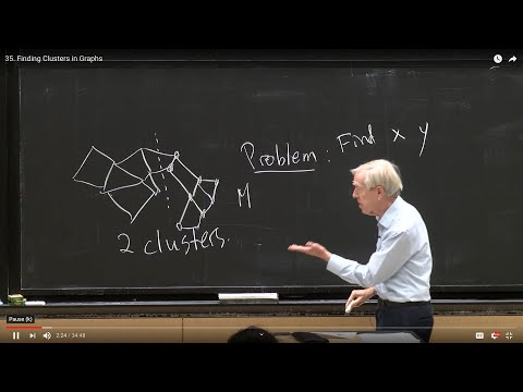
• Clustering objective: split the graph's nodes into two groups A and B with centers X and Y, minimizing the total squared distance from each point to its group's center, while keeping the groups reasonably balanced in size.
• Centroid: the best center for a fixed group of points is their centroid, the average of the points' position vectors.
• K-means algorithm: alternate between (1) computing centroids for the current groups and (2) reassigning each point to whichever centroid it is closer to, repeating until the clusters stop changing.
• Spectral clustering: uses the eigenvalues ("spectrum") of a matrix associated with the graph, specifically the graph Laplacian, to determine the clusters.
• Four key graph matrices: the incidence matrix A (edges by nodes, with -1/+1 entries), the degree matrix D (diagonal, counting edges at each node), the adjacency matrix (which nodes connect to which), and the graph Laplacian L = A^T A = D - (adjacency matrix).
• Laplacian properties: L is symmetric positive semi-definite; the all-ones vector is always an eigenvector with eigenvalue 0, and the name "Laplacian" comes from its resemblance to the discrete second-derivative (finite-difference) Laplace operator on a grid graph.
• Fiedler eigenvector: the eigenvector associated with the smallest positive eigenvalue of L (the second-smallest eigenvalue overall); named after Miroslav Fiedler.
• Clustering by sign: the two clusters in spectral clustering are formed from the nodes whose Fiedler eigenvector components are positive versus negative; because this eigenvector is orthogonal to the all-ones eigenvector, its positive and negative components balance out.

Walkthrough

Defining the clustering problem (0:00)

The lecture frames graph clustering as splitting nodes into two roughly balanced groups A and B, each represented by a center point (X and Y), to minimize the total squared distance from each node to its group's center.

K-means: the alternating partition algorithm (8:27)

Given a fixed partition, the best center for each group is shown to be its centroid (average position). The K-means algorithm alternates between computing centroids for the current clusters and reassigning each point to its nearest centroid, repeating until the clusters converge; the lecture notes this process lacks a guaranteed convergence rate but works well in practice.

Spectral clustering and the graph Laplacian (12:38)

The lecture introduces spectral clustering, named for its use of a matrix's eigenvalues ("spectrum"), and reviews the spectral theorem for symmetric matrices (real eigenvalues, orthogonal eigenvectors, with independent orthogonal eigenvectors for repeated eigenvalues). It defines the graph Laplacian L = A^T A, where A is the incidence matrix, and equivalently L = D - (adjacency matrix), walking through a small example graph to construct the incidence, degree, and adjacency matrices explicitly.

The Spectral Theorem and properties of L (14:05)

The lecture confirms that L is symmetric positive semi-definite and always has the all-ones vector as an eigenvector with eigenvalue 0, since L applied to a constant vector gives zero. It also connects the name "Laplacian" to the discrete second-difference structure seen on a grid graph, which mirrors the continuous Laplace equation.

The Fiedler eigenvector and forming clusters (23:37)

The lecture identifies the Fiedler eigenvector as the eigenvector for the smallest positive eigenvalue of L (excluding the trivial zero eigenvalue). Because this eigenvector is orthogonal to the all-ones vector, its positive and negative components balance, and the lecture explains that these signs are used to split the graph's nodes into the two clusters. It closes by noting that this approach can extend to more clusters by using several of the lowest eigenvectors, though quality typically degrades as the number of clusters grows.

Before you watch

• Be comfortable with eigenvalues and eigenvectors of symmetric matrices and the spectral theorem.
• Familiarity with basic graph terminology (nodes, edges, degree) is helpful for the Laplacian construction.
• Reviewing distance-based clustering ideas (centroids, minimizing squared distance) helps for the K-means section.

Check your understanding

1. What objective does K-means minimize, and why is the centroid the optimal center for a fixed group of points?
2. Describe the two alternating steps of the K-means algorithm.
3. How is the graph Laplacian constructed from the incidence matrix or from the degree and adjacency matrices?
4. Why does the graph Laplacian always have the all-ones vector as an eigenvector with eigenvalue 0?
5. How does the Fiedler eigenvector determine a two-way clustering of a graph's nodes?