Lecture 31: Eigenvectors of Circulant Matrices, the Fourier Matrix

What this lecture covers

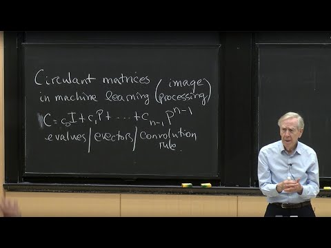
This lecture continues the study of circulant matrices from the previous lecture, first explaining why shift-invariant matrices (circulants and their non-cyclic cousins, Toeplitz matrices) matter in machine learning, and then working out their eigenvalues and eigenvectors. It builds toward the discrete Fourier transform, showing that the eigenvector matrix of any circulant is the Fourier matrix.

After watching, you can explain why convolutional structure reduces the number of weights a network needs to learn, identify which broad families of matrices (symmetric, orthogonal, anti-symmetric, normal) have orthogonal eigenvectors, and derive the eigenvalues and eigenvectors of the cyclic shift matrix as roots of unity.

Key ideas

• Why convolution matters for machine learning: an image with millions of pixels would need an impossibly large weight matrix if every weight were independent; convolution (constant-diagonal, shift-invariant weights) cuts this down to a number of weights proportional to n, not n^2.
• Circulant vs. Toeplitz: a circulant matrix has constant diagonals that wrap around cyclically (cyclic convolution); a Toeplitz matrix has constant diagonals without wrapping (ordinary convolution), which is the more common structure in practice.
• Max pooling: a separate, nonlinear operation that reduces image size by replacing a block of pixels with their maximum, distinct from the linear convolution operation.
• Eigenvalues of the cyclic shift matrix: for the n x n permutation matrix P, the eigenvalues are the n-th roots of unity, lambda^n = 1, equally spaced around the unit circle in the complex plane.
• Families with orthogonal eigenvectors: symmetric matrices (real eigenvalues), orthogonal matrices (eigenvalues of magnitude 1), anti-symmetric matrices (purely imaginary eigenvalues), and more generally normal matrices (M^T M = M M^T, or with complex conjugate transpose) all have orthogonal eigenvectors.
• Circulants are normal: because circulant matrices commute with each other, a circulant and its transpose commute, so circulants are normal matrices and hence have orthogonal eigenvectors.
• Shared eigenvectors: since every circulant is a polynomial in the shift matrix P, all circulants of a given size share the same eigenvectors, namely those of P.
• The Fourier matrix: the eigenvector matrix built from powers of W = e^(2*pi*i/n) is exactly the (unnormalized) discrete Fourier transform matrix, whose columns are orthogonal.

Walkthrough

Why circulant and Toeplitz matrices matter for machine learning (0:22)

The lecture opens with logistics on final projects, then motivates circulant and Toeplitz matrices: an image with millions of pixels would require an infeasibly large weight matrix per layer if computed naively, but shift-invariant (convolutional) weights need only n parameters instead of n^2. It distinguishes circulant matrices (cyclic convolution) from Toeplitz matrices (ordinary convolution, more typical in machine learning), and briefly contrasts this linear operation with the nonlinear max pooling step used to shrink images.

Discrete Fourier transform and circulant structure (2:25)

The lecture recalls that a circulant matrix is fully determined by its first row or column, and links this structure to the discrete Fourier transform, previewing that the same eigenvectors will appear across all circulants of a given size.

Eigenvalues of the cyclic shift matrix (19:13)

Starting from the permutation (cyclic shift) matrix P, the lecture computes its characteristic equation, finding lambda^n = 1. For the 4-by-4 case this gives eigenvalues 1, -1, i, -i; for the 8-by-8 case it gives the eight eighth-roots of unity, evenly spaced on the unit circle and labeled as powers of W = e^(2*pi*i/8).

Families of matrices with orthogonal eigenvectors (26:42)

To place P's eigenvectors in context, the lecture reviews matrix families known to have orthogonal eigenvectors: symmetric matrices (real eigenvalues), orthogonal matrices (eigenvalues on the unit circle, since they preserve vector length), and anti-symmetric matrices (purely imaginary eigenvalues, illustrated with a 90-degree rotation example). It then introduces normal matrices, M = Q * diag * Q^T with any eigenvalues but orthogonal eigenvectors, defined by the test that a matrix commutes with its transpose (or conjugate transpose for complex matrices).

Circulants are normal, and share eigenvectors (35:33)

The lecture shows that because any two circulant matrices commute, a circulant commutes with its own transpose, making it a normal matrix and guaranteeing orthogonal eigenvectors. Since every circulant is a polynomial in the shift matrix P, all circulants of a given size share P's eigenvectors.

Building the Fourier matrix (40:07)

The lecture constructs the eigenvector matrix explicitly: the first eigenvector is the all-ones vector (eigenvalue 1), and successive eigenvectors are powers of W, W^2, and so on, filling out a matrix whose entries are all powers of W. This matrix is identified as the Fourier matrix, and the lecture verifies for both an 8-by-8 and a 3-by-3 example that its columns are orthogonal, by showing that sums of the roots of unity cancel to zero.

Before you watch

• Watch the previous lecture on circulant matrices and cyclic convolution, which introduces the shift matrix P and the definition of a circulant.
• Review how to compute eigenvalues via the characteristic polynomial (det(A - lambda*I) = 0).
• Be comfortable with complex numbers and roots of unity on the complex plane.

Check your understanding

1. Why does using a convolution (shift-invariant) matrix instead of an arbitrary weight matrix make deep learning on images computationally feasible?
2. What is the difference between a circulant matrix and a Toeplitz matrix?
3. Why are the eigenvalues of the cyclic shift matrix P the n-th roots of unity?
4. What test identifies a normal matrix, and why does that guarantee orthogonal eigenvectors?
5. Why do all circulant matrices of a given size share the same eigenvectors, and what is that shared eigenvector matrix called?