Lecture 27: Backpropagation, Finding Partial Derivatives

What this lecture covers

This lecture opens with two suggested course projects based on Suvrit Sra's earlier stochastic gradient descent (SGD) lecture, then moves to its main topic: backpropagation, the algorithm used to compute the gradient of a neural network's loss efficiently. It follows directly from the previous lecture on the layered, composed structure of a neural network's learning function f(x).

After watching, you can explain what a computational graph is, why differentiating a chain of functions "in reverse" (from the output back to the inputs) is far cheaper than computing each partial derivative separately, and why the order of operations in a chained computation, whether differentiation or matrix multiplication, can change its cost by orders of magnitude.

Key ideas

• Project ideas from SGD: comparing sampling with and without replacement, and observing SGD's fast initial progress followed by oscillation near the optimum ("region of confusion"), are both offered as possible course projects.
• Early stopping: stopping training before fully converging is a deliberate strategy to avoid overfitting, tying back to SGD's typical behavior of getting close to the optimum quickly.
• Computational graph: a function built by composing simple steps (for example, x^3 times x + 3y) can be represented as a directed graph of intermediate operations, which is evaluated forward to compute the function's value.
• Chain rule on a graph: the derivative of a composed function is found by applying the chain rule, product rule, and power rule to each step of the graph in turn.
• Forward mode is wasteful: computing one partial derivative at a time (for example, only df/dx) forward through the graph requires a separate pass for each variable.
• Reverse-mode automatic differentiation (backpropagation): by propagating derivatives backward through the graph starting from the output, all partial derivatives can be obtained together at a small multiple (roughly three to five times) of the cost of one, instead of a separate computation per variable.
• Order of operations matters: multiplying a chain of matrices in different orders (A(BC) versus (AB)C) can differ enormously in computational cost, especially when one of the matrices is a vector; backpropagation implicitly chooses the cheap order for derivatives.

Walkthrough

Project ideas revisiting stochastic gradient descent (0:00)

The lecture suggests two possible course projects inspired by the previous guest lecture: empirically comparing convergence of an average when sampling with versus without replacement, and reproducing the characteristic SGD behavior of rapid early progress followed by oscillation near the optimum, tied to the idea of early stopping.

Setting up backpropagation (8:38)

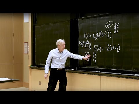
The lecture introduces backpropagation as the calculation needed to find the gradient of the loss function F efficiently, so that gradient descent can take a step. It credits the technique's role in making deep learning practical, noting it was also known earlier as automatic differentiation, and recalls the network's structure as a composition f(x) = f3(f2(f1(x))) from the previous lecture.

A worked example: computing the function (11:08)

Using the example function x^3 * (x + 3y), the lecture builds a computational graph with intermediate nodes and evaluates it forward for x = 2, y = 3, getting a final value of 88. This graph structure is then reused for computing derivatives.

Forward-mode differentiation and its cost (15:25)

Working through the chain rule by hand, the lecture computes df/dx step by step through the graph using the power rule and product rule, arriving at a value of 140. It notes that this same process would need to be repeated separately to get df/dy, which is the source of forward mode's inefficiency.

Reverse mode and its efficiency (26:59)

The lecture explains reverse-mode automatic differentiation: starting from df/df = 1 and working backward through the same graph, both df/dx and df/dy can be obtained from a single backward pass, reusing shared intermediate results. This is why the cost of getting a gradient with many variables (as in deep networks with millions of weights) is only a small multiple of computing the function itself, not proportional to the number of variables.

Order matters: matrix multiplication cost example (44:35)

To illustrate why computation order changes cost dramatically, the lecture compares multiplying three matrices A, B, C as A(BC) versus (AB)C, deriving the operation counts for each. When C is a column vector, multiplying A by B first is drastically more expensive than multiplying B by C first, illustrating why backpropagation's ordering of computations (analogous to always multiplying against a vector) is the efficient choice.

Before you watch

• Watch the previous lecture on the structure of neural nets, which introduces the network as a composition of affine layers and ReLU activations.
• Review the chain rule, product rule, and power rule from single- and multivariable calculus.
• Be comfortable with the cost of matrix-matrix and matrix-vector multiplication in terms of operation counts.

Check your understanding

1. Why is computing a gradient one partial derivative at a time (forward mode) inefficient for functions of many variables?
2. What is the key idea that lets reverse-mode automatic differentiation compute all partial derivatives in roughly the cost of one forward pass?
3. In the worked example, why does going backward through the computational graph reuse intermediate values that a forward-only approach would have to recompute?
4. Why does the order of matrix multiplication in a product like A(BC) versus (AB)C matter so much when one of the matrices is a vector?
5. How does the matrix multiplication ordering example relate to why backpropagation is efficient?