Lecture 19: Saddle Points Continued, Maxmin Principle

What this lecture covers

This lecture closes the discussion of saddle points from the Rayleigh quotient, then shifts into the statistics material that leads into deep learning: mean, expected mean, and the start of covariance. Along the way Strang uses a lab assignment on polynomial curve fitting to introduce overfitting concretely, connecting it back to the Vandermonde matrix from an earlier guest lecture.

The lecture sits at the hinge between the course's linear algebra content and its probability and optimization content. After watching, you should be able to identify a saddle point of a Rayleigh quotient using its eigenvalues, describe overfitting in terms of polynomial degree versus number of data points, and state the difference between the sample mean and the expected mean.

Key ideas

• Rayleigh quotient extremes: for a symmetric matrix S, the maximum and minimum of R(x) = x^T S x / x^T x are the largest and smallest eigenvalues, reached at the corresponding eigenvectors.
• Middle eigenvalues are saddle points: eigenvalues between the largest and smallest are saddle values of the Rayleigh quotient, where the gradient is zero but the point is neither a max nor a min.
• Maxmin principle: a middle eigenvalue can be expressed as the maximum, over all subspaces of the right dimension, of the minimum of the Rayleigh quotient restricted to that subspace - this is the basis of the interlacing theorem for eigenvalues.
• Overfitting via polynomial degree: fitting M data points with a degree M-1 polynomial gives an exact fit (zero error) but the resulting curve is typically wild; lower-degree fits leave some least-squares error but tend to generalize better.
• Vandermonde matrix and interpolation: the square matrix that arises from exact polynomial interpolation is the Vandermonde matrix, notorious for having a very large inverse and poorly scattered singular values.
• Sample mean vs. expected mean: the sample mean averages actual observed outcomes; the expected mean weights every possible outcome by its probability, without needing an experiment to have happened.
• Covariance as a matrix concept: when several experiments happen together, the natural summary of their variability is a matrix, not a single number - a preview of the covariance matrix introduced in the next lecture.

Walkthrough

Finishing saddle points with the maxmin principle (2:03)

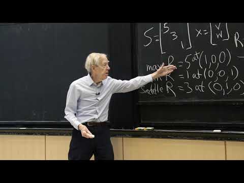
Using a diagonal 3x3 example with Rayleigh quotient values 5u^2 + 3v^2 + w^2 (normalized), Strang shows the maximum is 5, the minimum is 1, and the middle value 3 is a saddle point reached at the middle eigenvector. He then demonstrates the maxmin principle: restricting to a well-chosen 2D subspace and minimizing over it gives 3, and maximizing over all such subspaces still yields 3 - showing that a middle eigenvalue is the "max of the min" over subspaces of the right dimension.

Lab 3 and overfitting (20:40)

Strang walks through the class's curve-fitting lab: given six data points, a polynomial of degree 5 (six coefficients) fits them exactly, since the corresponding matrix A is square. He argues this exact fit is a natural example of overfitting - the curve passes through every point but behaves badly in between - and contrasts it with a straight-line fit, which underfits but is far more stable.

The Vandermonde matrix returns (27:54)

The square interpolation matrix that produces the exact polynomial fit is identified as the Vandermonde matrix, previously introduced in the guest lecture on numerically low-rank matrices. Strang notes its inverse is enormous and its singular values are widely scattered, which explains why exact high-degree interpolation is numerically unstable.

Sample mean and expected mean (40:23)

Moving into statistics, Strang distinguishes the sample mean, computed from actual trial outcomes and governed by the law of large numbers, from the expected mean, computed by weighting each possible outcome by its probability before any trial has occurred.

Sample variance and a first look at covariance (44:38)

Sample variance is introduced as the average squared distance from the sample mean, dividing by n-1. Strang then motivates covariance by describing what happens when two experiments (flipping two coins) are run together: independent coins give zero covariance, while coins glued together give maximal covariance, setting up the covariance matrix developed further in the next lecture.

Before you watch

• Review the Rayleigh quotient and how it relates to eigenvalues, covered earlier in this course.
• Recall the guest lecture on low-rank matrices, since the Vandermonde matrix's instability is revisited here.

Check your understanding

1. Why is a middle eigenvalue of a symmetric matrix a saddle point of its Rayleigh quotient rather than a maximum or minimum?
2. How does the maxmin principle express a middle eigenvalue using maximization and minimization over subspaces?
3. Why does fitting six data points exactly with a degree-5 polynomial count as overfitting, even though the error is zero?
4. What is the practical difference between the sample mean and the expected mean?