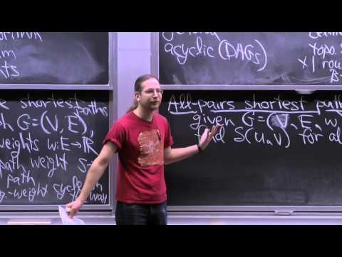
11. Dynamic Programming: All-Pairs Shortest Paths

What this lecture covers

The lecture answers a single question: given a directed graph with weighted edges (possibly negative), how do you find the shortest path between every pair of vertices, faster than just running a single-source algorithm from each vertex in turn? It follows the earlier lecture on dynamic programming and precedes further graph algorithms in MIT's 6.046 course, building on single-source shortest-path algorithms (BFS, Dijkstra, Bellman-Ford) that students are assumed to already know.

By the end, you can derive two dynamic-programming formulations of all-pairs shortest paths, connect one of them to matrix multiplication and repeated squaring, state and apply the Floyd-Warshall algorithm, and explain how Johnson's algorithm reweights edges so that Dijkstra can be run safely even when the original graph has negative edge weights.

Key ideas

• All-pairs vs. single-source: all-pairs shortest paths asks for the distance Delta(u, v) between every pair of vertices, not just from one source; it's motivated by pre-computing distances for fast repeated queries, such as a mapping service.
• Naive baseline: running a single-source algorithm from every vertex gives V^2 (BFS), V^2 log V + VE (Dijkstra), or V^2 E (Bellman-Ford); the last case can cost as much as V^4 in dense graphs.
• DP1 (edge-count parameterization): define d(u, v, m) as the shortest path from u to v using at most m edges, guess the last edge, and relax; this runs in V^4 time, no better than repeated Bellman-Ford.
• Relaxation: every shortest-path algorithm in the lecture repeatedly enforces the triangle inequality d(u,v) <= d(u,x) + d(x,v), updating d(u,v) downward when it's violated.
• Matrix multiplication connection: replacing + with min and * with + (a semiring the lecture calls 'circle world') turns the DP1 recurrence into circle-matrix multiplication, and repeated squaring computes it in V^3 log V.
• Floyd-Warshall: redefines subproblems as C(u, v, k), the shortest path using only intermediate vertices 1..k; guessing only whether vertex k is used (not where) gives a V^3 algorithm with no log factor.
• Johnson's algorithm: reweights edges using a height function h so all weights become non-negative, then runs Dijkstra from every vertex; the height function itself comes from running Bellman-Ford once from an added zero-weight source vertex.
• Negative-weight cycles: all-pairs algorithms can detect them (a negative value on the diagonal of the distance matrix, or Bellman-Ford failing to satisfy the difference constraints used to build Johnson's height function).

Walkthrough

Recap of single-source algorithms (0:00)

The lecture opens by reviewing the running times of single-source shortest-path algorithms across four scenarios: unweighted graphs (BFS, V+E), non-negative weights (Dijkstra, V log V + E), general weights (Bellman-Ford, VE), and DAGs (one pass of Bellman-Ford after a topological sort, linear time). These numbers become the baseline for comparison throughout the lecture.

Defining all-pairs shortest paths (7:06)

Delta(s, v) is defined as the weight of the shortest path from s to v, which can be infinite (no path) or negative infinity (a reachable negative-weight cycle). The all-pairs problem asks for Delta(u, v) for every pair, motivated by applications like pre-computing distances between major cities or routing tables, where queries need to be answered quickly and often.

Naive results and the target bound (11:13)

Running each single-source algorithm from every vertex gives baseline running times, the worst being V^2 E (up to V^4 in dense graphs) for general weights via Bellman-Ford. The lecture names Johnson's algorithm as the target: it matches the cost of running Dijkstra V times (V^2 log V + VE) even when the graph has negative weights, which is presented as a surprising result given that Dijkstra alone can't handle negative weights.

DP1: parameterizing by number of edges (15:25)

Following a five-step recipe for dynamic programs (subproblems, guessing, recurrence, acyclic order, final answer), the lecture defines d(u, v, m) as the shortest path from u to v using at most m edges. Guessing the last edge on the path gives the recurrence d(u,v,m) = min over x of d(u,x,m-1) + w(x,v), with base case d(u,u,0) = 0 and infinity otherwise. Written as nested loops, this is a relaxation step identical in spirit to Dijkstra and Bellman-Ford, and it runs in V^4 time — no improvement yet, but it sets up the next idea.

Matrix multiplication and repeated squaring (35:05)

The DP1 recurrence is shown to be exactly matrix multiplication if addition is replaced by min and multiplication by +. Under this reinterpretation, computing d(*, *, m) for all m up to n-1 is equivalent to computing w raised to a 'circle power'. Naively that takes n matrix multiplications (V^4 again), but repeated squaring reaches the same result in only log n multiplications, giving V^3 log V. The lecture notes this semiring lacks subtraction, so faster matrix-multiplication algorithms (Strassen and its successors) don't apply here, though they do apply to a related problem, transitive closure.

Floyd-Warshall algorithm (49:24)

A different subproblem definition removes the log factor. C(u, v, k) is the shortest path from u to v using only intermediate vertices numbered 1 through k. Instead of guessing which vertex comes last (n choices), the algorithm guesses only whether vertex k is used at all (2 choices): C(u,v,k) = min(C(u,v,k-1), C(u,k,k-1) + C(k,v,k-1)). This constant-time recurrence per subproblem yields a V^3 algorithm, described as about five lines of code and the standard choice for dense graphs.

Johnson's algorithm (59:48)

For sparse graphs, Johnson's algorithm gets closer to V^2 log V + VE. It reweights each edge (u,v) to w(u,v) + h(u) - h(v) for some height function h, chosen so all new weights are non-negative; the lecture proves that this reweighting shifts every path between two fixed endpoints by the same fixed amount, so shortest paths are preserved. Finding a valid h is shown to be equivalent to solving a system of difference constraints, which has a solution exactly when the graph has no negative-weight cycle. The construction adds a new source vertex with zero-weight edges to every other vertex, runs Bellman-Ford once from it to get h, reweights all edges, then runs Dijkstra from every vertex and translates the results back to the original weights.

Before you watch

• Know Dijkstra's algorithm, Bellman-Ford, and BFS for single-source shortest paths, and the definition of the triangle inequality for shortest-path weights.
• Be comfortable with the standard dynamic-programming recipe (subproblems, guessing, recurrence, base cases, evaluation order).
• Some familiarity with matrix multiplication and repeated squaring for exponentiation is useful for the middle section.

Check your understanding

1. Why does the naive DP1 formulation (parameterizing by number of edges used) take V^4 time, and what does redefining the subproblem in Floyd-Warshall change to bring that down to V^3?
2. In Johnson's algorithm, why must the height function h satisfy w(u,v) + h(u) - h(v) >= 0 for every edge, and how does the proof show that shortest paths are preserved under this reweighting?
3. Why does a negative-weight cycle make the system of difference constraints unsolvable, and how does the lecture use Bellman-Ford to detect this?
4. What property of the 'circle world' semiring (min-plus) prevents Strassen-style fast matrix multiplication from being applied to speed up the DP1/matrix-multiplication approach?