Lecture 9, Part 4: Natural Gradient and Trust Region Methods

What this lecture covers

This closing part of Lecture 9 introduces a second way to enforce closeness between successive policies: instead of a Lagrangian penalty, approximate the constrained optimization problem with a trust region, which leads to the natural policy gradient. The lecture shows why plain gradient ascent implicitly enforces the wrong kind of closeness constraint (in parameter space rather than distribution space) and derives the fix using a second-order approximation involving the Fisher information matrix.

This follows directly from the KL-divergence-constrained policy gradient of the previous part, and closes out the lecture's broader argument connecting policy gradient to policy iteration. It sets up methods such as natural policy gradient, TRPO, and PPO referenced throughout the rest of the course.

Key ideas

• Trust region idea: a first-order Taylor expansion of the true objective is only accurate near the current parameters, so optimizing the linear approximation only makes sense within a bounded "trust region."
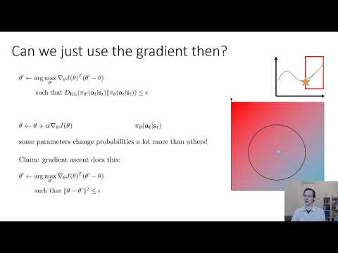
• Linearized objective, exact gradient: differentiating the importance-weighted advantage objective at theta' = theta recovers exactly the standard policy gradient, since the importance weights cancel.
• Gradient ascent's hidden constraint: plain gradient ascent solves a constrained problem too, but the constraint is Euclidean distance in parameter space, not KL divergence in distribution space, so it can silently violate the intended closeness bound when some parameters affect action probabilities far more than others.
• Fisher information matrix: a second-order Taylor expansion of the KL divergence around theta' = theta gives a quadratic form governed by the Fisher information matrix, which can be estimated from the same samples used for the policy gradient.
• Natural gradient: solving the trust-region problem with this quadratic KL approximation gives a closed-form update equal to the inverse Fisher information matrix times the standard gradient, correctly reshaping the step to respect distribution-space closeness.
• Why it matters in practice: in a simple Gaussian policy example, gradient ascent becomes severely ill-conditioned as the policy's variance shrinks, because the variance parameter affects probabilities much more strongly than the mean parameter; natural gradient corrects this.
• Practical algorithms: exact natural gradient requires computing the Fisher-inverse-gradient product, often via conjugate gradient; related practical algorithms include TRPO (computing a step size for a target KL) and PPO (using the Lagrangian-style penalty from the previous part).

Walkthrough

From constrained optimization to a trust region (0:00)

The lecture reframes the KL-constrained policy optimization problem as trust-region optimization: approximate the objective with its first-order Taylor expansion (which is just the gradient) and only trust that approximation within a bounded region, since without a constraint the linear approximation is unbounded.

Gradient ascent as the wrong trust region (6:13)

Differentiating the linearized objective at theta' = theta gives exactly the standard policy gradient. But applying vanilla gradient ascent implicitly solves a trust-region problem where the constraint is Euclidean distance in parameter space, not the intended KL divergence between the resulting policies. Because some parameters change action probabilities much more than others, this parameter-space constraint doesn't correctly approximate the distribution-space constraint, which is demonstrated with a Gaussian policy example where shrinking variance dominates the gradient and stalls progress on the mean.

Deriving the natural gradient (7:57)

To fix this, the lecture uses a second-order Taylor expansion of the KL divergence (the first-order term vanishes at theta' = theta), yielding a quadratic form governed by the Fisher information matrix, an expectation over grad log pi outer products that can be estimated from samples. Solving the trust-region problem with this quadratic constraint in place of the Euclidean one gives a closed-form update: the natural gradient, equal to the inverse Fisher information matrix times the standard policy gradient, with a step size chosen to satisfy the KL bound exactly.

Practical notes and algorithms (17:54)

Computing the natural gradient exactly requires the product of the inverse Fisher information matrix with the gradient, typically computed efficiently with conjugate gradient rather than by forming the full matrix, as done in trust region policy optimization (TRPO). The lecture closes by tying the lecture's ideas together: policy gradient is policy iteration with a state-distribution approximation that is valid when policies stay close; this closeness can be enforced with an explicit KL constraint (via a Lagrangian, as in the previous part) or an approximate trust region (via natural gradient, as in this part), and both ideas underlie practical algorithms such as TRPO and proximal policy optimization (PPO).

Before you watch

• Watch the previous part of Lecture 9 on the KL-divergence-constrained policy gradient objective and dual gradient descent, since this part offers an alternative way to enforce the same constraint.
• Basic familiarity with Taylor expansions and Lagrangian optimization is helpful for following the derivation.

Check your understanding

1. Why does optimizing a first-order Taylor expansion of the objective require a trust region rather than being unconstrained?
2. In what sense does vanilla gradient ascent enforce "the wrong constraint," and why does this matter for a Gaussian policy's mean and variance parameters?
3. What role does the Fisher information matrix play in deriving the natural gradient?
4. How do TRPO and PPO relate to the two ways of enforcing policy closeness discussed across this lecture?