Lecture 9, Part 2: Bounding the State Distribution Mismatch

What this lecture covers

This part closes the gap left at the end of Part 1 of Lecture 9: the proof that maximizing advantage under the old policy's state distribution approximates the true RL objective requires the old and new policies' state distributions to be close. The lecture proves this for both deterministic and stochastic policies, then bounds how much the resulting objective can differ from the true objective.

This continues directly from the previous part's derivation connecting policy gradient to policy iteration, and its result (a bound scaling with the total variation divergence between policies) motivates the constrained policy gradient methods introduced next.

Key ideas

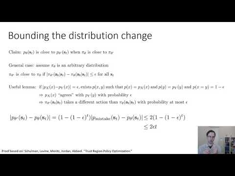
• Goal: show that the state marginal p_theta(s_t) is close to p_theta'(s_t) whenever the policies pi_theta and pi_theta' are close, so it's valid to substitute one for the other.
• Deterministic case: if the new policy has at most epsilon probability of deviating from the old one at each step, the state distribution splits into a "no mistake" branch (weight (1 - epsilon)^t, matching the old policy's distribution) and an unknown "mistake" branch, mirroring the imitation-learning bound from earlier in the course.
• Total variation bound: using (1 - epsilon)^t >= 1 - epsilon*t, the divergence between the two state distributions is bounded by 2 * epsilon * t.
• Stochastic case: a coupling lemma extends the same style of argument to stochastic policies, showing that if pi_theta and pi_theta' have total variation divergence at most epsilon, they take the same action with probability at least 1 - epsilon, giving the same 2 * epsilon * t bound on state marginals.
• From states to objective values: bounding the divergence of state distributions lets you bound the difference between expectations of any bounded function f(s_t) under the two distributions, with an error term of 2 * epsilon * t * max(f).
• Applying it to the RL objective: applied to the importance-weighted advantage, this shows the tractable objective is a lower bound on the true RL objective improvement, off by an error term of order epsilon * T * R_max (or epsilon * R_max / (1 - gamma) in the infinite-horizon case).
• Practical implication: as long as the new policy stays close enough to the old one (small epsilon), maximizing the tractable importance-weighted advantage objective is guaranteed to improve the true RL objective.

Walkthrough

Setting up the state-distribution bound (0:18)

The lecture restates the goal from Part 1: show p_theta(s_t) stays close to p_theta'(s_t) when pi_theta and pi_theta' are close, so that the importance-weighted advantage objective, differentiable to give exactly the policy gradient, approximates the true improvement in the RL objective.

Bounding the mismatch for deterministic and stochastic policies (1:23)

For a deterministic old policy, the new policy's state distribution at time t splits into a term where every action so far matched the old policy (probability (1 - epsilon)^t, same state distribution as the old policy) and an unconstrained "mistake" term, exactly paralleling the earlier imitation-learning bound. This gives a total variation bound of 2 * epsilon * t between the state marginals. The lecture then generalizes to stochastic policies using a coupling lemma from the trust region policy optimization paper: if two distributions have total variation divergence epsilon, a joint distribution exists under which they agree with probability at least 1 - epsilon, yielding the same style of bound.

Bounding the objective value (10:51)

The lecture extends the state-marginal bound to expectations of an arbitrary bounded function, showing that the expected value under the new policy's states is bounded below by the expected value under the old policy's states minus an error term proportional to epsilon, t, and the function's maximum value. Applying this to the importance-weighted advantage objective, and noting that an advantage is bounded by the horizon times the maximum reward, shows the constant in the error term is order T * R_max (or R_max / (1 - gamma) for infinite horizon with discounting). The conclusion is that maximizing the tractable, differentiable objective under the old policy's states is guaranteed to improve the true RL objective, provided the new and old policies stay close enough that epsilon is small.

Before you watch

• Watch Part 1 of Lecture 9, which sets up the claim this part proves and introduces the importance-weighted advantage objective.
• Recall the imitation learning bound on compounding errors from earlier in the course, since the deterministic-policy proof here follows the same structure.

Check your understanding

1. Why does the deterministic-policy proof split the new policy's state distribution into a "no mistake" and a "mistake" term?
2. What does the coupling lemma let you conclude about two stochastic policies whose total variation divergence is bounded by epsilon?
3. How does bounding the state marginal difference translate into a bound on the difference between the two policies' objective values?
4. What does this derivation imply about how large a policy update should be allowed to be?