Lecture 8, Part 6: Practical Tips and Q-Learning Case Studies

What this lecture covers

This closing part of Lecture 8 gives practical advice for implementing Q-learning, useful directly for the course's homework, and then surveys papers that apply the techniques covered across the lecture: replay buffers, target networks, double Q-learning, n-step returns, and continuous-action Q-learning.

After watching you can list concrete debugging and tuning practices for Q-learning, and place several well-known papers (from early auto-encoder-based fitted Q-iteration through DQN, DDPG, and parallel robotic Q-learning) within the lecture's conceptual framework.

Key ideas

• Debug on easy problems first: verify correctness on simple, reliable tasks before tuning hyperparameters on the real problem, since Q-learning is more finicky than policy gradient methods.
• Stability varies by task: across Atari games some (like Pong) train very consistently across random seeds while others (like Venture) sometimes fail entirely; larger replay buffers (around 1 million transitions) tend to improve stability.
• Exploration and patience: performance can stay near random for a long time before improving; start with high epsilon and anneal it as the Q-function improves.
• Clip large gradients or use Huber loss: a squared-error Bellman objective can produce huge gradients from very bad actions whose exact value doesn't matter; Huber loss behaves like clipped gradients but is often easier to implement.
• Use double Q-learning and Adam: double Q-learning is simple, generally helps, and has little downside; adaptive optimizers like Adam outperform older choices like RMSProp.
• Run multiple seeds: Q-learning results vary a lot between random seeds, so multiple runs are needed to confirm a result rather than a lucky or unlucky fluke.

Walkthrough

Practical tips for Q-learning (0:17)

The lecture recommends debugging on simple, known-solvable problems first, notes that stability differs dramatically across Atari games, and highlights large replay buffers as a reliable stability booster. It also stresses patience, since Q-learning can stay near random performance for a long stretch before improving, and recommends scheduling exploration from high to low epsilon.

Advanced tips for Q-learning (2:41)

Large Bellman errors from clearly bad actions can dominate the gradient even though their exact value is unimportant; gradient clipping or a Huber loss addresses this. Double Q-learning is described as nearly free to add and generally beneficial. N-step returns help especially early in training but introduce bias for larger n. Adam is recommended over older optimizers, and running several random seeds is essential given how inconsistent Q-learning results can be.

Case studies in Q-learning research (5:14)

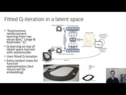
The lecture walks through several papers: an early (2012) system that runs fitted Q-iteration with extra-random trees on an auto-encoder's latent space to control a slot car; the original DQN paper using convolutional networks with replay buffers, target networks, and one-step backups; the DDPG paper for continuous-action robotic control using a learned maximizer network; a paper on real-world robotic door-opening using the NAF architecture with multiple parallel robots; and a large-scale grasping system that instantiates the lecture's three-process (data collection, target update, learning) view of Q-learning across many parallel workers.

Suggested readings and recap (9:32)

The lecture points to classic and deep RL readings, including Watkins's original Q-learning paper, the neural fitted Q-iteration paper, the DQN paper, the double Q-learning paper, the DDPG-style approximate-maximizer paper, the NAF paper, and dueling network architectures (a discrete-action analogue of NAF not covered in the lecture). It closes with a recap of the lecture: replay buffers and target networks for stability, the unified three-process view of Q-learning, double Q-learning, multi-step returns, and continuous-action Q-learning via sampling, analytic optimization, or a learned actor network.

Before you watch

• Complete the earlier parts of Lecture 8 covering replay buffers, target networks, double Q-learning, n-step returns, and continuous-action Q-learning, since this part assumes and reviews all of them.

Check your understanding

1. Why does the lecture recommend debugging Q-learning on easy problems before tuning hyperparameters on the target task?
2. What problem does a Huber loss (or gradient clipping) solve in Q-learning, and why does it arise?
3. Why is it important to run multiple random seeds when evaluating a Q-learning result?
4. How does the large-scale robotic grasping system relate to the three-process view of Q-learning described earlier in the lecture?