Lecture 8, Part 3: A Unified View of Q-Learning

What this lecture covers

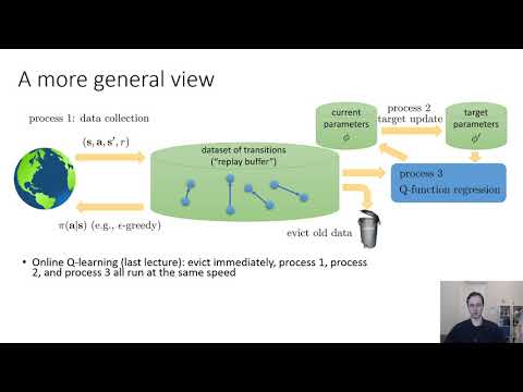
This short segment steps back from the specific Q-learning variants covered so far and asks how fitted Q-iteration, online Q-learning, and DQN with replay buffers and target networks relate to each other. It reframes them as one general algorithm expressed as parallel processes running at different speeds.

After watching, you can describe Q-learning as three (or four, including buffer eviction) processes acting on a shared replay buffer, and explain each prior algorithm as a particular choice of how fast each process runs.

Key ideas

• Shared replay buffer: the buffer of transitions is the central object that every version of Q-learning reads from and writes to.
• Process 1 (data collection): continuously runs the current policy (for example epsilon-greedy on phi) in the environment and appends new transitions to the buffer.
• Eviction process: keeps the buffer bounded, typically as a ring buffer that discards the oldest transition when a new one arrives.
• Process 2 (target update): periodically copies phi into the target parameters phi', either by a hard copy or Polyak averaging, and normally runs much more slowly than the other processes.
• Process 3 (learning): samples a batch, computes targets using phi', and updates phi by gradient descent.
• Algorithms as rate choices: online Q-learning is the case where the buffer holds only one transition and all processes run in lockstep; DQN runs data collection and learning at the same rate with a slow, large-buffer target update; fitted Q-iteration nests learning inside target updates inside data collection.
• Non-stationarity control: running the processes at different rates is what keeps each process's view of the problem close to stationary, which is why the separation helps convergence.

Before you watch

• Watch the earlier parts of Lecture 8 on replay buffers and target networks, since this section reframes those exact mechanisms.

Check your understanding

1. What are the three (or four) processes in the unified Q-learning view, and what does each one do?
2. How does online Q-learning correspond to a specific choice of buffer size and process rates?
3. Why does running process 2 much more slowly than process 3 help stabilize learning?
4. How does fitted Q-iteration fit into this framework as nested loops?