Lecture 5, Part 5: Implementing Policy Gradients in Practice

What this lecture covers

This part turns the policy gradient math into something you can actually code with automatic differentiation tools. It answers: how do you get PyTorch or TensorFlow to compute the policy gradient efficiently, without manually calculating a gradient vector for every sampled state-action pair?

After watching, you can write a "pseudo-loss" that tricks an autodiff package into producing the correct policy gradient, and you know practical settings — batch size, learning rate, optimizer — to expect when training with policy gradients.

Key ideas

• Why naive computation is expensive: computing grad log pi(a|s) separately for every sampled state-action pair produces a vector as long as the number of network parameters (often millions) for each of potentially thousands of samples, which is costly in memory and compute.
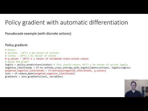
• Pseudo-loss trick: instead of the real objective, implement J-tilde, the sum of log-probabilities of sampled actions weighted by their reward-to-go (Q-hat); this quantity isn't the RL objective itself, but its gradient equals the policy gradient.
• Reuse of maximum-likelihood code: log pi is the same cross-entropy loss (discrete actions) or squared error (Gaussian continuous actions) used in supervised learning; policy gradient implementation just multiplies per-sample likelihoods by precomputed reward-to-go values before taking the mean and calling backward.
• Autodiff doesn't need to know Q-hat depends on theta: the reward-to-go values are treated as fixed weights, not differentiated through, which is what makes the trick work.
• High variance changes practice: despite looking like supervised learning, policy gradient training needs much larger batch sizes (thousands to tens of thousands of samples) because gradients are noisy.
• Optimizer and tuning: plain SGD with momentum is hard to use; Adam is a reasonable default, and expect more hyperparameter tuning than typical supervised learning, with dedicated step-size methods like natural gradient covered later.

Before you watch

• Watch the earlier parts of this lecture on deriving the policy gradient, causality, baselines, and off-policy importance sampling.
• Be familiar with how automatic differentiation and backpropagation work in a deep learning framework.

Check your understanding

1. Why is computing grad log pi separately for every sampled state-action pair computationally expensive?
2. What is the pseudo-loss J-tilde, and why does its gradient equal the true policy gradient even though it isn't the RL objective itself?
3. How does implementing a policy gradient differ from implementing a standard maximum-likelihood loss?
4. Why do policy gradient methods typically need much larger batch sizes than supervised learning?