Lecture 5, Part 2: Intuition and the High-Variance Problem

What this lecture covers

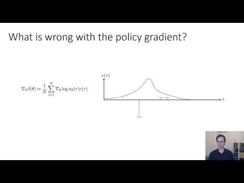
This part builds intuition for the policy gradient formula derived earlier in the lecture and shows why it doesn't work well out of the box. It compares the policy gradient to maximum likelihood training, extends the derivation to continuous actions, notes that the derivation carries over to partially observed problems, and then demonstrates a core weakness: the policy gradient estimator has high variance.

After watching, you can explain the policy gradient as a reward-weighted version of maximum likelihood, write the log-probability gradient for a Gaussian policy, and describe why adding a constant to the rewards can change the estimated gradient for a finite sample even though it shouldn't change the optimal policy.

Key ideas

• Weighted maximum likelihood: grad log pi is the same term used in supervised maximum likelihood training; policy gradient multiplies it by trajectory reward, so it raises the log-probability of high-reward trajectories and lowers it for low-reward ones, instead of always raising it.
• Discrete actions: log pi is simply the log probability the network assigns to the chosen discrete action.
• Continuous actions: representing pi_theta(a|s) as a Gaussian with a neural-network mean gives a closed-form gradient, -1/2 * Sigma^-1 * (s - a) * d(mean)/d(theta), computed by backpropagation.
• Trial-and-error formalized: the policy gradient can be read as gradient ascent that makes "good" trajectories more likely and "bad" ones less likely, formalizing trial-and-error learning.
• Partial observability: the derivation never used the Markov property, so the same policy gradient formula applies unchanged to observations instead of states in partially observed problems.
• High variance: with a small number of samples, shifting all rewards by a constant (which should not change the optimal policy) can visibly change the estimated gradient direction, because it changes which samples get their probability raised versus lowered; this variance shrinks only as sample count grows.

Before you watch

• Watch the previous part of this lecture, which derives the policy gradient formula and the REINFORCE algorithm.
• Know the Markov property and how it differs between states and observations.

Check your understanding

1. How does the policy gradient differ from the maximum likelihood gradient used in supervised learning?
2. Why does adding a constant offset to all rewards leave the optimal policy unchanged in theory, but still change the estimated gradient with a small sample?
3. Why does the policy gradient derivation extend to partially observed problems without modification?
4. What is the closed-form gradient of the log probability for a Gaussian policy with a network-predicted mean?