Lecture 4: Introduction to RL Algorithms, Part 2

What this lecture covers

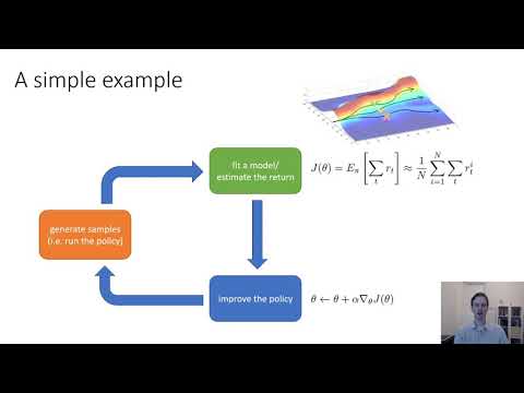
This short lecture describes the high-level structure common to nearly all reinforcement learning algorithms covered in the course: a loop of generating samples, estimating something about the current policy, and improving the policy, and discusses which of these steps tend to be computationally expensive.

After watching, you should be able to name the three boxes in the RL algorithm anatomy, give an example of each for a simple policy gradient method and a model-based method, and explain what makes sample generation cheap or expensive.

Key ideas

• Three-part anatomy: every RL algorithm in the course generates samples (orange box) by running the policy in the environment, fits a model or estimate (green box) of how well the policy is doing, and improves the policy (blue box) — then repeats.
• Policy gradient example: the green box simply sums rewards along sampled trajectories; the blue box computes a policy gradient and takes a gradient step, making good trajectories more likely and bad ones less likely.
• Model-based example ("RL by backprop"): the green box trains a full dynamics model f_phi(s_t, a_t) ≈ s_{t+1} via supervised learning; the blue box backpropagates through the model and reward to optimize the policy directly.
• Cost of the orange box (sampling): collecting trajectories from a real-world system (robot, car, power grid) can be extremely expensive and slow, while simulators like MuJoCo can run at up to 10,000x real time, making sampling nearly free.
• Cost of the green and blue boxes varies too: summing rewards or taking a single gradient step is cheap; training an entire dynamics model or backpropagating through a model and policy can be expensive.
• Different algorithms emphasize different boxes: for example, Q-learning (covered later) concentrates most computation in the green box, with a cheap argmax as its blue box.

Before you watch

• Watch Lecture 4 Part 1 first for the MDP and RL objective definitions this framework builds on.

Check your understanding

1. What are the three boxes in the shared anatomy of RL algorithms, and what does each one do?
2. How does the green box differ between a simple policy gradient method and a model-based "RL by backprop" method?
3. Why might the cost of the orange (sampling) box vary so much between a real robot and a MuJoCo simulator?
4. In what sense does Q-learning concentrate its effort mostly in the green box?