Lecture 19, Control as Inference, Part 3

What this lecture covers

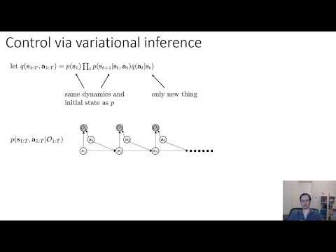
This part addresses the optimism problem identified with exact inference in the control-as-inference graphical model: because the backward pass conditions on high reward, it can bias transition probabilities toward lucky outcomes, like inferring that a lottery player is likely to win just because they hold a winning ticket. The lecture fixes this using the variational inference tools from the previous week, constraining the approximate posterior to keep the true dynamics fixed while only learning the action distribution.

By the end, you should be able to explain why exact inference distorts the dynamics, describe how restricting the variational distribution to match the true transitions and initial state removes this bias, and derive the resulting objective, which turns out to be the standard expected-reward RL objective plus an action-entropy bonus, optimized with a soft version of value iteration.

Key ideas

• Optimism problem: exact inference under the optimality-variable model computes p(a_t | s_t, O_{1:T}), which effectively asks "given you got lucky, what did you do", not "what would you have done to be optimal", biasing the inferred behavior toward risky, high-variance outcomes.
• Restricted variational distribution: define q(s_{1:T}, a_{1:T}) to use the true initial state distribution and true transition probabilities, but let only q(a_t|s_t) be learned, matching the graphical model with the optimality nodes removed.
• Resulting lower bound: because the initial-state and transition terms cancel between p and q, the evidence lower bound simplifies to the expected sum of rewards plus the entropy of the action distribution at each timestep.
• Interpretation: maximizing this bound is exactly the standard RL objective (maximize expected reward) plus an entropy bonus that rewards stochastic, near-optimal behavior, explaining the "suboptimal monkey" behavior from part 1.
• Exponential-of-quantity solution rule: whenever an objective has the form "expected value of something minus the log probability of the distribution it's taken under," the optimal distribution is proportional to the exponential of that quantity.
• Soft value iteration backward pass: from the last timestep backward, set Q_t = r_t + E[V_{t+1}] (the ordinary, non-optimistic Bellman backup) and V_t = log integral of exp(Q_t) (a soft max), with the resulting policy q(a_t|s_t) = exp(Q_t - V_t).
• Variants: a discount factor gamma can be added (equivalent to a probability of "death" each step), and a temperature alpha can interpolate between soft and hard max; the same recursion also has a valid infinite-horizon version.

Before you watch

• Watch parts 1 and 2 of this lecture, which introduce the optimality-variable graphical model and its exact-inference backward pass, including the optimism problem this part resolves.
• Review the variational inference lectures (evidence lower bound and the general recipe for approximating a posterior with a restricted distribution class), since this part directly reuses that machinery.

Check your understanding

1. Why does exact inference in the optimality-variable model bias the inferred policy toward risky actions, using the lottery-ticket analogy?
2. What specific restriction on the variational distribution q prevents the optimism bias, and why does that restriction make the lower bound simplify so cleanly?
3. How does the resulting variational lower bound relate to the standard reinforcement learning objective, and what extra term does it add?
4. Why does the rule "optimal distribution is the exponential of the expected quantity" apply here, and what does it say the optimal q(a_T|s_T) looks like at the final timestep?