Lecture 15: Training Large Models

What this lecture covers

This lecture addresses two linked scaling problems for training deep networks: fitting a model's memory footprint onto a single GPU, and spreading training across multiple devices. It sits after the course's GPU programming material and treats GPU memory hierarchy as background already covered.

After watching, you should be able to explain why training costs more memory than inference, describe activation checkpointing and why it gives sublinear memory cost, and distinguish model-parallel from data-parallel training, including the allreduce and parameter-server abstractions used to implement data parallelism.

Key ideas

• GPU memory hierarchy: consumer GPUs commonly offer 8-10 GB of global memory while server cards like the A100 offer 40-80 GB, and model size is frequently bottlenecked by this global memory.
• Sources of memory consumption: weights, optimizer state (e.g. momentum), intermediate activation values, and input data all consume GPU memory during training.
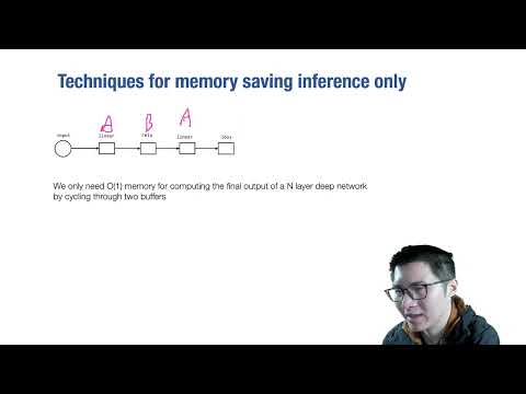
• Inference memory reuse: for inference-only feed-forward networks, activations can be cycled through two ping-pong buffers, so memory cost stays constant regardless of network depth.
• Why training costs more: backward-pass gradients depend on forward-pass activations, so those activations can't be freed early, giving naive training an O(n) memory cost in the number of layers.
• Activation checkpointing: store only a subset of activations ("checkpoints") during the forward pass, discard the rest, and recompute short segments on demand during the backward pass; checkpointing every sqrt(n) layers yields O(sqrt(n)) memory at roughly 25% extra compute.
• Model parallelism: partition the computational graph itself across workers, inserting send/receive pairs at the boundaries; pipeline parallelism with micro-batches keeps workers busy concurrently.
• Data parallelism: replicate the full model on every worker, split a mini-batch across workers, compute gradients independently, then combine them.
• Allreduce and parameter server: allreduce sums a value across all workers and returns the sum to everyone; a parameter server instead collects gradients centrally, applies updates, and can tolerate slow or dead workers by proceeding with whichever gradients have arrived.

Walkthrough

GPU memory hierarchy and sources of memory consumption (1:49)

The lecture recaps GPU memory hierarchy, noting the gap between consumer cards (8-10 GB) and server cards (40-80 GB), and lists the sources of memory use during training: model weights, optimizer state, intermediate activations, and input data.

Memory-saving techniques for inference vs. training (6:55)

For inference-only networks, activations can be recycled through two alternating buffers regardless of network depth, since each layer's output is only needed by the next layer. Training breaks this trick because backward-pass gradient computation for each layer needs that layer's forward-pass activation, so a naive implementation must keep O(n) activations alive for an n-layer network.

Activation checkpointing (14:57)

The lecture introduces checkpointing: store only selected ("colored") activations during the forward pass and discard the rest, then during the backward pass recompute a short forward segment to refill a deleted activation just before it's needed for gradient computation. Checkpointing every k layers costs O(n/k) for the checkpoints plus O(k) for each recomputation segment; choosing k = sqrt(n) gives O(sqrt(n)) total memory, at roughly 25% additional compute since only one extra forward pass is required overall.

Model-parallel and pipeline-parallel training (26:56)

When a single model doesn't fit on one device, the computational graph can be partitioned across workers, with send/receive operations inserted at partition boundaries. Because a single micro-batch leaves most workers idle, pipeline parallelism runs multiple micro-batches concurrently so different workers process different micro-batches at the same time, keeping the pipeline busy.

Data-parallel training via allreduce and parameter server (32:32)

Data parallelism replicates the model on every worker and splits a mini-batch across them. The allreduce abstraction sums each worker's local gradient array element-wise across all workers and returns the total to every worker, requiring no change to the model code itself. The parameter-server alternative sends gradients to a central server that sums and applies updates, which allows it to proceed without waiting for every worker and simplifies recovery when a worker restarts.

Overlapping communication with computation (41:05)

Because gradients for later layers become available before earlier-layer gradients finish computing, their communication (via allreduce or parameter server) can be overlapped with ongoing backward computation, and prioritized based on when each layer's updated weight is next needed. The lecture closes by summarizing model versus data parallelism and pointing to further techniques such as Microsoft's ZeRO for advanced memory sharing.

Before you watch

• Review the course's GPU programming lecture, particularly the GPU memory hierarchy and shared/global memory distinction.
• Be familiar with how automatic differentiation builds a computational graph and computes gradients via backward passes.

Check your understanding

1. Why can inference reuse just two buffers regardless of network depth, while naive training cannot?
2. How does choosing a checkpoint interval of k = sqrt(n) lead to O(sqrt(n)) memory cost, and what is the compute trade-off?
3. What is the key structural difference between allreduce-based and parameter-server-based data parallel training?
4. Why does overlapping communication with computation matter for data-parallel training speed?