Lecture 8: Continuous Random Variables

What this lecture covers

This lecture opens a new unit in MIT 6.041 on continuous random variables, translating the discrete-case toolkit (PMFs, expectation, variance) into the continuous setting. It defines the probability density function, explains why individual points have zero probability, and introduces the cumulative distribution function (CDF) as a notation that unifies discrete and continuous (and mixed) random variables. The lecture closes by introducing the normal distribution and the standardization trick used to compute normal probabilities from a table.

After watching, you'll be able to interpret a density function, compute probabilities as areas under a density curve, relate a CDF to its density by differentiation, recognize mixed random variables, and standardize any normal random variable to look up probabilities from the standard normal table.

Key ideas

• Density functions replace PMFs: probability of X falling in [a,b] is the area under the density curve, integral from a to b of f(x) dx, the continuous analog of summing a PMF.
• Individual points have zero probability: for continuous random variables, P(X=a) = 0, so the density value itself is not a probability.
• Density is probability per unit length: for small delta, P(x <= X <= x+delta) ≈ f(x) * delta, so densities can exceed 1 as long as the total area is 1.
• Expectation and variance carry over by analogy: sums become integrals and PMFs become PDFs, but the center-of-mass interpretation and the variance shortcut formula still hold.
• The CDF unifies discrete and continuous cases: F(x) = P(X <= x) is continuous and increases smoothly for continuous random variables, but jumps in a staircase for discrete ones, with jump sizes equal to point probabilities.
• The density is the derivative of the CDF, wherever that derivative exists.
• Mixed random variables combine a discrete point mass with a continuous spread, and only the CDF describes them cleanly.
• The normal distribution is centered at mu with spread controlled by sigma; linear functions of normal random variables are themselves normal.
• Standardizing a normal random variable, (X - mu) / sigma, turns it into a standard normal so its probabilities can be read from a single table.

Walkthrough

Densities and the definition of a continuous random variable (0:00)

The lecture sets up continuous random variables as taking values anywhere on the real line, and explains that probability mass, instead of sitting in discrete chunks, is spread continuously and described by a density function. A random variable is continuous if probabilities over intervals equal the area under a density curve, mirroring the discrete PMF sum but with an integral.

Probabilities of small intervals (10:09)

Looking at a small interval [x, x+delta], the lecture shows the probability of landing in it is approximately f(x) * delta, which is why the density is described as probability per unit length rather than a probability itself, and why densities are allowed to exceed 1.

Area under the curve and unions of intervals (11:01)

The lecture confirms that densities must be non-negative and integrate to 1 over the whole real line, and shows how to extend interval probabilities to unions of intervals by adding the separate integrals.

Expectation and variance for continuous variables (13:06)

Expectation is defined by replacing the PMF sum with a density integral, keeping the center-of-gravity interpretation. The expected value of a function of X can be computed directly from X's density without first finding the distribution of g(X), and variance keeps its usual shortcut formula. The uniform random variable is worked as an example, giving mean (a+b)/2 and variance (b-a)^2/12.

The cumulative distribution function (15:28)

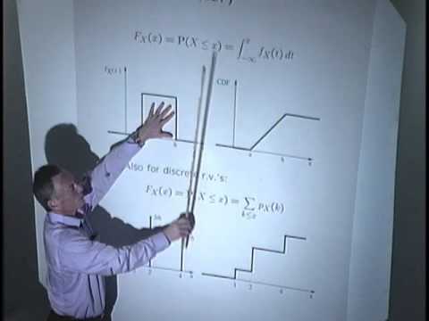
The CDF F(x) = P(X <= x) is introduced as a single concept that applies to both discrete and continuous random variables. For continuous variables it's found by integrating the density from -infinity to x and is itself continuous and increasing; for discrete variables it's a staircase that jumps at each point with positive probability mass, and the density (where it exists) is the derivative of the CDF.

Mixed random variables (23:30)

A random variable can combine a discrete point mass with a continuous spread, illustrated by a game that pays a fixed amount with some probability and a uniformly random amount otherwise. Such a mixed random variable is neither purely discrete nor purely continuous, but its CDF is still well defined, showing a jump where the point mass sits and continuous growth elsewhere.

Parsing the normal density formula (33:56)

The lecture builds up the standard normal density from exp(-x^2/2), explaining why the tails fall off quickly and why the 1/sqrt(2*pi) constant is needed to make the density integrate to 1. It generalizes to a normal centered at mu with spread sigma, and explains that a linear function of a normal random variable is itself normal, with mean and variance transforming in the usual linear way.

Standardizing and using the normal table (41:40)

Since the normal CDF has no closed form, probabilities are read from a table of the standard normal. Any normal random variable can be standardized via (X - mu) / sigma, giving a standard normal whose CDF values are tabulated, which the lecture demonstrates with a worked probability calculation.

Before you watch

• Review PMFs, expectation and variance for discrete random variables from the earlier chapters of this course.
• Be comfortable with basic integration and the idea of area under a curve.
• Know the binomial distribution, since the lecture previews its connection to the normal distribution.

Check your understanding

1. Why does a continuous random variable assign zero probability to every individual point?
2. How do you recover the density function from a given CDF, and where might this fail?
3. Why is a mixed random variable neither discrete nor continuous, and how does its CDF reflect that?
4. Explain why standardizing a normal random variable produces a standard normal, and why this is useful for computing probabilities.