Lecture 16: Markov Chains I

What this lecture covers

This lecture opens a new topic, Markov chains, after finishing Bernoulli and Poisson processes. It answers the question of how to model random systems where the future depends on the current state but not on the full history, using a supermarket checkout queue as a running example. Unlike the memoryless processes covered earlier, Markov chains let the state itself carry dependence across time.

The lecture builds up the formal definition of a discrete-time, finite-state Markov chain, states the Markov property precisely, derives a recursion for computing n-step transition probabilities, and works a two-state numerical example that reveals a chain settling into steady-state probabilities. It closes by introducing the structural classification of states as recurrent or transient, setting up further structural analysis for the next lecture.

Key ideas

• State: the state must capture everything about the present that is relevant for predicting the future; choosing it correctly is what makes the Markov property hold (for example, a moving ball's state needs both position and velocity, not position alone).
• Markov property: given the current state, the probability of moving to any other state next is fixed and does not depend on how the process arrived at the current state.
• Transition probabilities p_ij: the one-step conditional probability of moving from state i to state j, which together with the state diagram fully specify the chain.
• Supermarket queue example: customer arrivals modeled as a Bernoulli process with parameter p and service completions as geometric with parameter q, giving a finite state space (queue length from 0 to a capacity limit) with transitions up, down, or unchanged.
• n-step transition probability r_ij(n): the probability of being at state j after n steps starting from i, computed by a recursion that conditions on the state one step before (or after) the target time, using the total probability theorem.
• Steady-state behavior: in the worked two-state example, the n-step probabilities converge to fixed values (2/7 and 5/7) regardless of the starting state, illustrating that randomness can wash out the effect of the initial state.
• Periodicity blocks convergence: a chain with a strict alternating pattern between states never settles to a limit; the n-step probability keeps oscillating.
• Recurrent vs transient states: a state is recurrent if, from it, there is always a way back regardless of where the chain goes; it is transient if there is some reachable state from which return is impossible. Transient states are visited only finitely many times before the chain settles into a recurrent class.

Walkthrough

Introducing Markov processes and the queue example (0:40)

The lecture frames Markov processes as a generalization of physical evolution equations with randomness added, then sets up a checkout-counter queue: customer arrivals follow a Bernoulli process with parameter p, and service completions follow a geometric distribution with parameter q, both modeled as independent coin flips.

Defining the state and transition diagram (7:20)

The queue length becomes the state, truncated to a maximum capacity, giving a finite set of states. The lecture enumerates the possible one-step transitions (arrival only, departure only, both, or neither) and their probabilities, noting that boundary states (empty or full queue) have modified transition rules.

The Markov property and choosing the state (14:38)

The lecture states the Markov property formally: the transition probability out of a state does not depend on the path used to reach it. It stresses that defining the state correctly, so that it captures all relevant information, is what makes this property hold, using a flying ball's position and velocity as an illustration of an incomplete versus complete state.

General setup and n-step transition recursion (18:27)

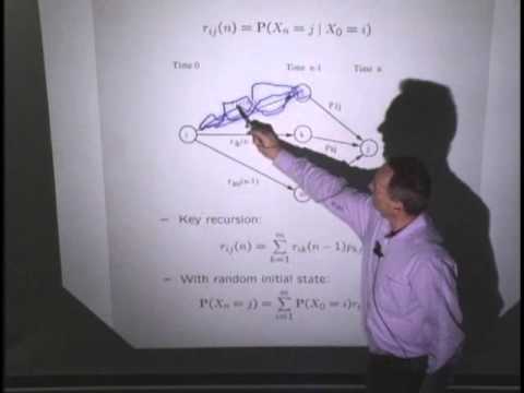
The lecture generalizes to any finite-state, discrete-time Markov chain, defines r_ij(n) as the n-step transition probability, and derives a recursion for it using the total probability theorem by conditioning on the state one step before (or after) the endpoint, relying on the Markov property to justify treating each intermediate state independently of how it was reached.

Worked two-state example (25:49)

Using a chain with two states and given transition probabilities, the lecture computes the n-step probabilities by hand for successive values of n and observes them converging to 2/7 and 5/7, independent of the starting state. This illustrates the idea of a steady state: the state itself keeps changing, but the probabilities describing it stabilize.

When convergence fails: periodicity (42:25)

A chain that strictly alternates between two states every step never converges: the probability of being back at the starting state is 1 after an even number of steps and 0 after an odd number. This periodic structure is identified as the key obstruction to convergence.

Recurrent and transient states (46:04)

The lecture defines a state as recurrent if, from it, every reachable state has a path back, and transient otherwise. It works through a diagram identifying recurrent and transient states, explains that a chain will eventually leave its transient states permanently and settle into a class of recurrent states, and notes that when a chain has multiple separate recurrent classes, the initial state determines which class it gets stuck in.

Before you watch

• Review the Bernoulli process (geometric inter-arrival times) and basic conditional probability, since the queue example depends on both.
• Be comfortable with the total probability theorem, used repeatedly to derive the n-step transition recursion.
• Have a working understanding of what a probability distribution over states means, since this lecture shifts from arrival counts to state probabilities.

Check your understanding

1. Why must the state of a system include velocity as well as position for the Markov property to hold for a flying ball?
2. In the supermarket queue example, why do the transition probabilities change at the boundary states (empty and full queue)?
3. How does the total probability theorem lead to the recursion for n-step transition probabilities?
4. Why does a chain with strict two-state alternation fail to converge to steady-state probabilities?
5. What distinguishes a recurrent state from a transient state, and why do transient states get visited only finitely often?