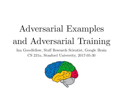
Lecture 16: Adversarial Examples and Adversarial Training

What this lecture covers

Guest lecturer Ian Goodfellow addresses a puzzle that only became interesting once deep learning started working well: carefully crafted, visually imperceptible changes to an input can make a trained network confidently misclassify it. The lecture explains what adversarial examples are, why they exist, how they threaten real systems, what defenses have been tried, and how the same techniques can improve machine learning even without a real adversary.

By the end, you can explain why adversarial examples arise from models being too linear rather than too complex, describe the fast gradient sign method and why it works, and explain why adversarial examples transfer between different models and datasets. You will also understand why most proposed defenses fail, why adversarial training is one of the few approaches with a real effect, and how the same optimization process appears in model-based optimization for engineering design.

Key ideas

• Adversarial example: an input deliberately perturbed by a small, often imperceptible amount so that a model misclassifies it with high confidence.
• Linearity hypothesis: adversarial examples arise mainly because deep networks (especially with ReLUs) are close to piecewise linear functions of their input, which extrapolate in unreasonable ways far from the training data.
• Fast gradient sign method (FGSM): a fast attack that perturbs each input pixel by a fixed amount in the direction of the sign of the gradient of the training cost with respect to the input.
• Adversarial subspace: adversarial perturbations occupy a contiguous, many-dimensional region (found to be around 25 dimensions on MNIST) rather than isolated points, which is why nearby perturbations also fool the model.
• Transferability: adversarial examples crafted for one model frequently fool other models, including different architectures and models trained on different data, which enables black-box attacks against systems the attacker cannot directly query.
• Clever Hans metaphor: machine learning models, like the horse Clever Hans, can appear to solve a task by picking up on cues that do not generalize once the shortcut is removed.
• Adversarial training: training on a mix of clean and adversarially perturbed examples that reduces vulnerability to the same class of attack and can also improve accuracy on the original clean task.
• Model-based optimization: using a trained network to search for inputs that maximize some predicted property (e.g. a fast car design) runs into the same failure mode as adversarial examples, since the optimizer finds inputs the model overrates rather than inputs that are actually good.

Walkthrough

Why adversarial examples matter now (1:10)

The lecture opens by noting that deep learning reached roughly human-level performance on several vision tasks around 2013, which made unexpected mistakes newly interesting to study. It introduces the panda-to-gibbon example: a nearly invisible, carefully computed perturbation flips a confident correct classification into an even more confident wrong one, and traces the history of such attacks back to work on fooling spam detectors and early results by Battista Biggio and Christian Szegedy.

Turning objects into airplanes (7:16)

An early visualization experiment shows that running gradient ascent on an image to maximize a target class's probability does not make the image look like that class. Instead, it finds a fooling image nearly indistinguishable from the original. The lecture generalizes this to simple linear models, showing an MNIST digit swept through all 10 classes by small perturbations while still looking like the original digit to a human.

Why linearity explains the failure (12:20)

Two competing explanations are tested: overfitting (random, model-specific mistakes) versus underfitting from excessive linearity. Evidence against overfitting includes that different models misclassify the same adversarial examples and that the same perturbation direction fools many clean examples. The lecture argues that deep networks with ReLUs are largely piecewise linear from input to output, and shows a 1D cross-section of a convolutional network's logits extrapolating linearly far from the data, which produces confident but wrong predictions.

The fast gradient sign method and adversarial subspaces (21:32)

FGSM is introduced as a first-order Taylor approximation attack constrained by a max-norm bound on the perturbation, achieving over 99% attack success on undefended networks. Decision boundary maps built from FGSM directions show that adversarial regions are contiguous and roughly linear, not isolated points, and follow-up work estimates these adversarial subspaces span around 25 dimensions on MNIST, which also explains why the same perturbation transfers across models.

Clever Hans, "wrong almost everywhere," and RL attacks (34:43)

The Clever Hans story frames how models can latch onto cues that generalize on natural test data but fail catastrophically under adversarial shift. The lecture shows that models classify almost all of input space incorrectly, not just a thin sliver, illustrated with Gaussian noise images confidently (and wrongly) labeled as specific classes. It also demonstrates adversarial perturbations against a reinforcement learning agent playing Atari Seaquest, showing the same attack framework degrades RL policies.

Transferability and real-world attacks (48:51)

The lecture covers black-box attacks: an attacker without access to a target model's weights can train a substitute model, either on their own labeled data or on queried outputs from the target, and adversarial examples crafted against the substitute transfer to the target. Ensembling multiple substitute models further boosts transfer success. Real demonstrations include fooling hosted classifiers from MetaMind, Amazon, Google, and Clarifai, fooling malware detectors, and fooling a camera-based object recognizer with printed photographs of adversarial images.

Defenses and adversarial training (1:00:03)

Most proposed defenses fail under stronger attacks; the lecture cites work showing many published defenses are broken. Simple generative modeling of the input distribution is not sufficient, since what matters is the posterior distribution over labels, which can still extrapolate linearly. Adversarial training, adding perturbed versions of training examples with their original labels, is shown to measurably reduce error on the same attack type and, for CIFAR-10 in one experiment, also improved clean-test accuracy by acting as a regularizer. Virtual adversarial training extends this to unlabeled data for semi-supervised learning.

Model-based optimization (1:08:10)

The lecture closes by connecting adversarial examples to model-based optimization: using a trained network's gradients to search for inputs (such as car blueprints or drug molecules) that maximize a predicted property tends to produce adversarial examples that fool the model rather than genuinely optimal designs. Solving the adversarial robustness problem is framed as a prerequisite for reliably using neural networks to guide engineering search.

Before you watch

• Review how gradients are computed and used for training (backpropagation), since the same machinery is used here to compute gradients with respect to the input image instead of the weights.
• Familiarity with softmax classifiers and cross-entropy loss from earlier lectures is assumed.
• Basic exposure to linear and logistic regression is useful, since several examples build the attack directly from a linear model's weights.

Check your understanding

1. Why does the lecture favor the linearity explanation for adversarial examples over the earlier overfitting explanation?
2. How does the fast gradient sign method use the sign of the input gradient to construct a perturbation, and why is the max-norm constraint important?
3. What does it mean for adversarial examples to "transfer," and why does this let an attacker fool a model they cannot directly query?
4. Why does simply modeling the input distribution with a generative model fail to defend against adversarial examples?
5. How does model-based optimization run into the same failure mode as adversarial attacks when searching for inputs that maximize a predicted property?