Lecture 8: Bias, Variance, and Model Selection

What this lecture covers

After several lectures on individual learning algorithms, this lecture turns to practical advice for making any of them work well. It explains the bias-variance tradeoff behind underfitting and overfitting, introduces regularization as the main tool for controlling overfitting, and gives it a Bayesian interpretation via maximum a posteriori (MAP) estimation. The second half covers how to split data into training, development, and test sets, when to use k-fold or leave-one-out cross-validation instead, and how forward search can select a useful subset of features.

After watching, you can diagnose whether a model is underfitting or overfitting, explain what regularization does mathematically and why it helps, and choose an appropriate way to split or cross-validate your data depending on dataset size.

Key ideas

• High bias (underfitting): a model too simple to capture the trend in the data, such as fitting a straight line to clearly curved data.
• High variance (overfitting): a model so flexible that it fits noise in the specific training sample, and would produce a very different fit on a different sample of similar data.
• Regularization: adding a penalty term like lambda * ||theta||^2 to the optimization objective, which discourages large parameter values and makes overfitting harder; lambda too large causes underfitting.
• MAP estimation: choosing parameters that maximize P(theta|S) under a prior P(theta); assuming a zero-mean Gaussian prior on theta produces exactly the regularization term seen with squared-norm penalties.
• Train/dev/test split: fit each candidate model on the training set, select the best one using error on a separate development (or cross-validation) set, and report unbiased performance only on a held-out test set never used for tuning.
• Dev/test set size: classic rules of thumb like 60/20/20 apply to small datasets; with very large datasets, the dev and test fractions shrink because a smaller absolute number of examples is still enough to distinguish algorithm performance.
• k-fold cross-validation: split the training data into k parts, train on k-1 and evaluate on the remaining one, repeat k times, and average the results; more data-efficient than a single dev split but k times more expensive to compute.
• Leave-one-out cross-validation: the extreme case of k-fold with k equal to the number of examples, used only for very small datasets.
• Forward search: a feature-selection method that starts with an empty feature set and greedily adds the single feature that most improves dev-set performance at each step.

Walkthrough

Bias and variance: underfitting vs. overfitting (5:10)

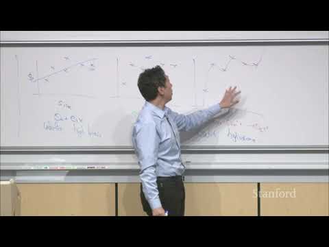
Using a housing price example, the lecture fits a straight line, a quadratic curve, and a fifth-order polynomial to the same small dataset. The straight line misses the visible curve in the data (high bias, underfitting); the fifth-order polynomial passes through every point but clearly doesn't generalize (high variance, overfitting); the quadratic fit sits in between. The same pattern appears in classification, where a decision boundary that's too simple or too complex mirrors the same underfitting and overfitting behavior.

Regularization (13:23)

To curb overfitting, the lecture adds a penalty term, lambda * ||theta||^2, to a model's optimization objective. Increasing lambda from 0 shrinks the fitted parameters and smooths the model's fit; setting lambda far too large forces parameters toward zero and causes underfitting instead. The same idea applies to logistic regression and other generalized linear models by subtracting the penalty from the objective being maximized. The lecture also notes that regularization is why an SVM can generalize well even while implicitly using an infinite-dimensional feature space: minimizing ||w||^2 keeps the margin large and the effective function class simple.

Bayesian interpretation of regularization (MAP estimation) (28:55)

Regularization can also be derived from a Bayesian point of view. Rather than finding the parameters that maximize P(S|theta) (maximum likelihood, the frequentist approach), MAP estimation finds the parameters that maximize the posterior P(theta|S), which by Bayes' rule is proportional to P(S|theta) * P(theta). Assuming a zero-mean Gaussian prior over theta and working through the algebra reproduces exactly the same squared-norm regularization term derived earlier, connecting the practical technique to a principled probabilistic justification.

Model complexity and the train/dev/test split (40:28)

As model complexity increases, training error keeps falling, but generalization error follows a U-shape: it decreases and then rises again as the model overfits. To find the sweet spot, and to choose things like polynomial degree, lambda, or an SVM's C parameter, the lecture recommends splitting data into a training set and a separate development set. Each candidate model is fit on the training set and evaluated on the development set, and the model with the best development-set error is selected; picking based on training-set error alone always favors the most complex model. A model's reported final performance should come from a third, untouched test set, since choices already tuned to the dev set make dev-set error an optimistically biased estimate.

Choosing dev and test set sizes (53:49)

Classic rules of thumb, such as 70/30 or 60/20/20 splits, work well for small to moderate datasets. With very large datasets, the lecture argues for allocating a much smaller percentage, sometimes just 1 to 5 percent, to dev and test, because that still provides enough absolute examples to reliably detect meaningful differences between algorithms. The guiding principle is to make dev and test sets large enough to distinguish the size of performance difference you actually expect to see between candidate models, and no larger than necessary.

K-fold and leave-one-out cross-validation (1:03:57)

When data is scarce, holding out a large dev set wastes valuable training examples. K-fold cross-validation addresses this by splitting the training set into k equal parts, training on k-1 of them and testing on the remaining part, repeating this k times so every part serves as the held-out set once, and averaging the resulting errors to score each candidate model. Ten-fold cross-validation is the most common choice. Leave-one-out cross-validation is the extreme case with k equal to the number of examples, used only when the dataset is very small, since it requires refitting the model once per example.

Feature selection via forward search (1:17:25)

When many available features are suspected to be irrelevant, such as most words in a spam-classification vocabulary, feature selection can reduce overfitting by keeping only the most useful ones. Forward search starts with an empty feature set, tries adding each remaining feature one at a time, keeps whichever single addition most improves development-set performance, and repeats until adding more features stops helping. This greedy procedure is computationally expensive but provides a practical way to narrow down a large feature set.

Before you watch

• Review linear regression, logistic regression, and the SVM's soft-margin objective from earlier lectures, since regularization and model selection are illustrated using all three.
• Recall the SVM's parameter C and locally weighted regression's bandwidth parameter tau, both mentioned as examples of hyperparameters chosen via the same dev-set procedures.
• Basic familiarity with Bayes' rule is useful for following the MAP estimation derivation.

Check your understanding

1. How can you tell from a model's training and validation error whether it is suffering from high bias or high variance?
2. Why does increasing the regularization parameter lambda eventually cause underfitting, and what happens if lambda is set to 0?
3. Why is it invalid to select a model using training-set error, and why is dev-set error also considered a biased estimate of true performance?
4. When would you prefer leave-one-out cross-validation over standard k-fold cross-validation, and what is the main cost of doing so?