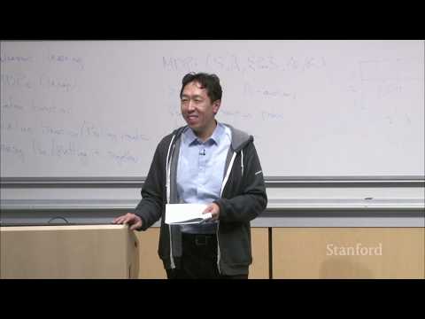
Lecture 17: MDPs, Value Iteration and Policy Iteration

What this lecture covers

This lecture answers the question left open in the previous session: given a Markov decision process, how do you actually compute the optimal policy? It builds up the machinery step by step, defining the value function for a fixed policy, deriving Bellman's equation for it, defining the optimal value function, and then presenting two algorithms, value iteration and policy iteration, that compute it.

The lecture then moves from the idealized setting, where the state transition probabilities are known, to the practical one, where they must be estimated from a robot's experience. It closes with a well-known difficulty in reinforcement learning: the tension between exploiting what the agent already believes is the best policy and exploring to discover better options, illustrated with epsilon-greedy exploration and a real-world example from online advertising. After watching, you should be able to derive Bellman's equation, implement value iteration or policy iteration for a small discrete-state MDP, and explain why an exploration strategy is needed on top of a greedy policy.

Key ideas

• Value function V_pi: the expected total discounted payoff of starting in a state and following policy pi from then on.
• Bellman's equation: V_pi(s) = R(s) + gamma * sum_s' P(s, pi(s), s') V_pi(s'), expressing a state's value as its immediate reward plus the discounted expected value of the next state.
• Solving for V_pi directly: for a fixed policy and a finite number of states, Bellman's equation is a linear system with one equation and one unknown per state, solvable exactly with a linear algebra solver.
• Optimal value function V*: V*(s) = max_pi V_pi(s), and it satisfies its own Bellman equation with a max over actions instead of a fixed policy.
• Value iteration: repeatedly applying the optimal-value Bellman equation to an initial guess (often all zeros) converges geometrically fast to V*, after which the optimal action at each state is the argmax over actions of the equation's right-hand side.
• Policy iteration: alternates between solving the linear system for the current policy's value function and updating the policy to be greedy with respect to that value function, converging in a finite number of steps to the exact optimal policy.
• Estimating transition probabilities: when P(s, a) is unknown, it is estimated from observed frequencies of ending up in each next state after taking each action, with a simple heuristic (uniform probability) for state-action pairs never observed.
• Exploration versus exploitation: a purely greedy policy can get stuck exploiting a known reward and never discover a better one; epsilon-greedy exploration takes a random action with small probability epsilon to keep exploring the state space.

Walkthrough

Recap: MDPs and the roadmap for finding an optimal policy (2:49)

The lecture recaps the five-tuple MDP definition from before and the 11-state grid-world example, then frames the day's goal: since the number of possible policies grows exponentially with the number of states, brute-force search is infeasible, so the lecture will define the value function V_pi, the optimal value function V*, and the optimal policy Pi* in order, then derive an efficient way to compute them.

The value function and Bellman's equation (11:38)

V_pi(s) is defined as the expected total discounted payoff of starting in state s and executing policy pi. The lecture derives Bellman's equation by splitting this expectation into the immediate reward received on waking up in s plus the discounted expected value of whatever state comes next, arriving at V_pi(s) = R(s) + gamma * E[V_pi(s')]. For a small MDP this turns into a linear system: with 11 states there are 11 equations in 11 unknowns, solvable directly with a linear algebra solver instead of iterating.

Defining the optimal value function (22:44)

The lecture defines V*(s) as the maximum of V_pi(s) over every possible policy, and derives a second Bellman equation for it that replaces the fixed policy with a max over actions: the best expected payoff from state s is the immediate reward plus the discounted value of the best next state reachable by any action. This equation immediately gives a recipe for the optimal action at each state, Pi*(s) = argmax_a of that same expression, once V* is known.

Value iteration (36:17)

Value iteration initializes an estimate of V to zero for every state and repeatedly applies the optimal-value Bellman equation as an update rule, either synchronously (updating all states at once from the previous estimate) or asynchronously (updating states one at a time using freshly updated values). Both variants converge, and with a discount factor like 0.99 the error shrinks geometrically each iteration, so a few hundred iterations bring the estimate very close to V*. The lecture works a concrete example, computing the expected future reward of moving west versus north from a given state using the converged V*, and shows west wins.

Policy iteration (53:04)

Policy iteration takes the opposite approach: it initializes a policy randomly, solves the linear system for that policy's exact value function, then updates the policy greedily with respect to that value function, and repeats. Unlike value iteration, which approaches V* asymptotically without ever reaching it exactly, policy iteration converges to the exact optimal policy in a finite number of iterations. It is efficient for small state spaces where solving the linear system is cheap, but value iteration scales better to large state spaces because it avoids repeatedly inverting a large system.

Estimating unknown transitions and exploration versus exploitation (59:00)

For a real robot, the state transition probabilities are usually unknown and must be estimated from observed frequencies of outcomes after taking each action in each state, with unseen state-action pairs defaulting to a uniform distribution over next states; the lecture notes that MDP solvers, unlike naive Bayes, are not very sensitive to these estimates being imperfect. The resulting loop, act, estimate transitions, solve for a new policy, repeat, converges to a good policy but has a blind spot: a purely greedy policy can settle on a known reward and never discover a better one elsewhere. This exploration-versus-exploitation trade-off, illustrated with online advertising as well as robotics, motivates epsilon-greedy exploration, where the agent follows its current policy most of the time but takes a random action with probability epsilon to keep discovering the state space; the lecture notes this always converges to the optimal policy for a discrete-state MDP, though possibly slowly.

Before you watch

• Review the MDP five-tuple (states, actions, state transition probabilities, discount factor, reward function) and the grid-world example from the previous lecture in this course.
• Be comfortable with expectations of random variables and with solving small linear systems of equations.
• Recall how gradient descent converges asymptotically, since the lecture draws a direct comparison to how value iteration approaches V*.

Check your understanding

1. How does Bellman's equation let you set up and solve for V_pi as a linear system rather than iterating?
2. What is the difference between the Bellman equation for V_pi and the one for V*, and how does the second one give you the optimal action directly?
3. Why does policy iteration reach the exact optimal policy in finitely many steps while value iteration only approaches V* in the limit?
4. When state transition probabilities are unknown, how are they estimated from a robot's experience, and what happens for state-action pairs never observed?
5. Why can a purely greedy policy fail to find the best available reward, and how does epsilon-greedy exploration address this?