Lecture 3: Building an MLP Character-Level Language Model

What this lecture covers

The previous lecture's bigram model only looked at one character of context, and scaling that counting approach to more context makes the probability table explode exponentially. This lecture answers the question of how to use more context without that blow-up, by implementing a multilayer perceptron (MLP) character-level language model based on Bengio et al. 2003. It is the third video in the makemore series, following directly from the bigram model built in lecture two.

By the end, you can build a small neural language model that takes several characters of context, embeds them in a lower-dimensional space, passes them through a hidden layer, and predicts the next character. Along the way the lecture introduces core PyTorch mechanics (indexing, view, broadcasting), the standard classification loss F.cross_entropy, minibatch training, learning rate search, and the train/dev/test split methodology used to detect underfitting and overfitting.

Key ideas

• Context explosion: counting-based models need a probability table whose size grows exponentially with context length, which is why more than one or two characters of context becomes impractical without a different approach.
• Embedding lookup table: each character (or word, in the original paper) is mapped to a point in a lower-dimensional vector space; these embeddings start random and are learned by backpropagation.
• Indexing as a linear layer: indexing into an embedding table with C[X] is mathematically equivalent to one-hot encoding the input and multiplying by C, but far more efficient.
• view vs cat: reshaping a tensor with .view() is nearly free because it only changes how the same underlying storage is interpreted, unlike torch.cat, which allocates new memory.
• F.cross_entropy: preferred over manually computing softmax and negative log likelihood because it fuses operations for speed and is numerically stable (it subtracts the max logit internally to avoid overflow).
• Minibatches: training on small random subsets of the data per step gives a noisier but much cheaper gradient estimate, letting you take many more steps per second than using the full dataset.
• Learning rate search: trying a range of learning rates (spaced exponentially) and plotting loss against them reveals a "good" range before the loss becomes unstable or explodes.
• Train/dev/test splits: an 80/10/10 split separates parameter training, hyperparameter tuning, and a final, rarely-used performance check, and comparing train vs. dev loss tells you whether a model is underfitting or overfitting.

Walkthrough

The problem with bigrams and the Bengio et al. 2003 paper (1:48)

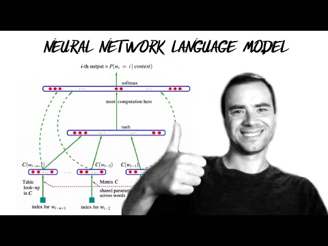
The lecture opens by reviewing why the bigram model breaks down: taking three characters of context already produces around 20,000 possible context rows, and the table quickly becomes too sparse. To fix this, the lecture turns to the Bengio et al. 2003 paper, which proposes embedding each vocabulary item into a continuous space (30 dimensions for 17,000 words in the original paper) and learning those embeddings jointly with the rest of the network via backpropagation. The intuition given is that words used in similar contexts end up with similar embeddings, letting the model generalize to phrases it never saw during training. The paper's diagram is walked through: an embedding lookup table C, a fully connected hidden layer with a tanh nonlinearity, an output layer sized to the vocabulary, and a softmax to turn the output into a probability distribution.

Building the training dataset (9:03)

A new notebook is started, reusing the vocabulary and character-to-integer mappings from the previous lecture. A block_size variable sets the context length (three characters, matching the paper's example). For each word, a sliding window of previous characters (padded with a special dot token) forms the input X, and the next character forms the label Y. Testing on just the first five words shows how the context window rolls forward one character at a time.

Embedding lookup table and hidden layer internals (12:19)

The embedding table C starts as 27 rows (one per character) by 2 columns, initialized randomly. Indexing C[X] embeds an entire batch of integer contexts at once, thanks to PyTorch's flexible indexing with lists, tensors, and multi-dimensional index arrays. To feed embeddings into the hidden layer, the three per-character embedding vectors need to be concatenated into a single row; the lecture shows a naive way with torch.cat and torch.unbind, then a far more efficient way using .view(), which reshapes the tensor without copying memory because it only manipulates the tensor's storage offset, strides, and shape. The hidden layer weights W1 and biases B1 are applied, followed by tanh, producing activations bounded between -1 and 1.

Output layer, cross-entropy loss, and training loop (29:15)

A second linear layer (W2, B2) maps the hidden activations to 27 output logits, one per possible next character. The manual softmax-plus-negative-log-likelihood calculation from the previous lecture is replaced with F.cross_entropy, which is faster, more numerically stable (it internally offsets logits by their maximum value to avoid overflow), and has a simpler analytic backward pass. The basic training loop is then assembled: zero the gradients, call loss.backward(), and nudge each parameter by learning_rate * grad. Training on just the first 32 examples shows the network can nearly memorize them (overfitting a single small batch), though the loss can't reach exactly zero because some contexts map to more than one valid next character.

Finding a good learning rate (45:40)

Once the full dataset (228,000 examples) is used, training all examples every step is too slow, so the lecture switches to random minibatches of 32 examples using torch.randint, which makes optimization nearly instant per step and gives a noisier but still useful gradient direction. To pick a learning rate rather than guessing, the lecture sweeps learning rates exponentially between roughly 0.001 and 1, tracks the resulting loss, and plots loss against the learning rate's exponent. The "valley" of that plot, around an exponent of -1 (a learning rate of about 0.1), gives a reasonable value. Training for thousands of steps with this learning rate, then decaying it by a factor of ten later in training, already surpasses the bigram model's loss.

Train/dev/test splits and diagnosing under/overfitting (53:20)

The lecture warns that a lower training loss alone doesn't mean a better model, since a large enough network can simply memorize the training set. The standard fix is splitting data into training (about 80%), dev/validation (about 10%), and test (about 10%) sets: training updates parameters, the dev set is used to compare hyperparameter choices, and the test set is checked only rarely at the very end. Comparing training and dev loss on the first model shows they're roughly equal, meaning the small network (about 3,400 parameters) is underfitting rather than overfitting.

Scaling up the network and sampling names (1:00:49)

To address underfitting, the hidden layer is enlarged (first to 300 neurons, later paired with a 10-dimensional embedding and 200 hidden neurons), and training is rerun with tuned learning rates. The two-dimensional character embeddings are visualized as a scatter plot, showing vowels clustering together and unusual characters like q and the dot token sitting apart, evidence the network has learned meaningful structure. After more tuning, the lecture reaches a best validation loss of 2.17 (down from the bigram model's 2.45), leaves further improvement as an exercise, and finishes by sampling new names from the trained model, which now produces noticeably more name-like output than the bigram model.

Before you watch

• Watch the previous lecture on bigram language models first; this lecture builds directly on its notebook, vocabulary, and loss formulation.
• Basic familiarity with matrix multiplication and PyTorch tensors will make the view/broadcasting discussion easier to follow.
• It helps to have seen backpropagation implemented from scratch (as in the micrograd series) since this lecture leans on loss.backward() without re-deriving it.

Check your understanding

1. Why does a counting-based bigram (or trigram) model become impractical as you increase the amount of context?
2. What does calling .view() on a tensor actually change, and why is it so much cheaper than torch.cat?
3. Why is F.cross_entropy preferred over manually computing softmax and negative log likelihood?
4. What do the training and dev/validation losses being roughly equal tell you about a model, and what's the usual fix?
5. How does the learning rate search method used in this lecture help you choose a learning rate?